Effect of Pd impurity on charge and spin density in metallic iron ...
Effect of Pd impurity on charge and spin density in metallic iron ...
Effect of Pd impurity on charge and spin density in metallic iron ...

You also want an ePaper? Increase the reach of your titles
YUMPU automatically turns print PDFs into web optimized ePapers that Google loves.
2 σ + 3 parameters at most provided the c<strong>on</strong>centrati<strong>on</strong> <str<strong>on</strong>g>of</str<strong>on</strong>g> impurities c is treated as variable.<br />
Otherwise the maximum number <str<strong>on</strong>g>of</str<strong>on</strong>g> variables describ<strong>in</strong>g distributi<strong>on</strong> equals 2 ( σ + 1)<br />
.<br />
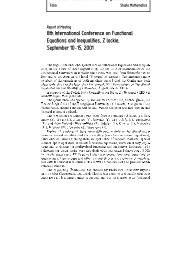
Figure 2.<br />
Hyperf<strong>in</strong>e field <strong>and</strong> relative spectral shift plotted versus palladium c<strong>on</strong>centrati<strong>on</strong>. Straight<br />
l<strong>in</strong>es are the lowest order approximati<strong>on</strong>s to the trends observed, particularly for shifts.<br />
Table III<br />
Essential results obta<strong>in</strong>ed with<strong>in</strong> b<strong>in</strong>omial distributi<strong>on</strong> model with σ = 3. The last row shows<br />
the averages <str<strong>on</strong>g>of</str<strong>on</strong>g> respective columns, where appropriate.<br />
c<br />
[at. %]<br />
< B > 3<br />
[T]<br />
± 0.02<br />
(3)<br />
B 0<br />
[T]<br />
± 0.02<br />
∆B 1<br />
[T]<br />
± 0.02<br />
∆B 2<br />
[T]<br />
± 0.02<br />
∆B 3<br />
[T]<br />
± 0.02<br />
< S<br />
> 3<br />
[mm/s]<br />
± 0.002<br />
0 32.97 0<br />
(3)<br />
S 0<br />
[mm/s]<br />
± 0.002<br />
∆S 1<br />
[mm/s]<br />
± 0.002<br />
∆S 2<br />
[mm/s]<br />
± 0.002<br />
∆S 3<br />
[mm/s]<br />
± 0.002<br />
0.95 33.18 32.96 1.66 0.95 0.61 0.008 0.006 0.015 0.011 0.006<br />
2.76 33.55 33.07 1.28 1.05 0.68 0.023 0.018 0.015 0.011 0.005<br />
4.71 33.87 33.17 1.39 0.97 0.38 0.035 0.026 0.018 0.014 0.004<br />
6.63 34.20 32.86 1.41 0.97 0.92 0.045 0.042 0.004 0.003 0.001<br />
8.04 34.50 33.00 1.37 1.14 0.85 0.052 0.047 0.007 0.004 0.001<br />
10.59 34.67 32.98 1.16 1.19 0.58 0.065 0.061 0.003 0.003 0.002<br />
33.01 1.38 1.05 0.67<br />
Figure 3 shows distributi<strong>on</strong> <str<strong>on</strong>g>of</str<strong>on</strong>g> the hyperf<strong>in</strong>e field <strong>and</strong> total shift encountered <strong>in</strong> some <str<strong>on</strong>g>of</str<strong>on</strong>g> the<br />
<strong>in</strong>vestigated samples. C<strong>on</strong>tributi<strong>on</strong>s from sub-spectra hav<strong>in</strong>g relative <strong>in</strong>tensities lesser than<br />
6