Diploma - Max Planck Institute for Solid State Research

– Photoemission on EuRh 2 Si 2 –
disentanglement of surface and bulk
structures
Diplomarbeit
zur Erlangung des akademischen Grades
Diplom-Physiker
vorgelegt von
Marc Höppner
geboren am 16.11.1986 in Großröhrsdorf
Institut für Festkörperphysik
Fachrichtung Physik
Fakultät Mathematik und Naturwissenschaften
Technische Universität Dresden
2011

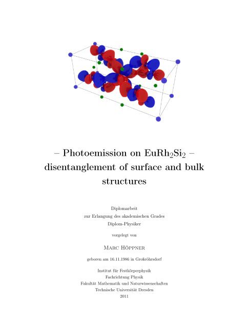
The Wannier function depicted on the cover page is
mainly based on Europium 4f z(x 2 −y 2 ) and Rhodium
4d z 2 illustrating a likely hybrid orbital in EuRh 2 Si 2 .
It is the Fourier transformed Bloch band with Europium
4f z(x 2 −y 2 ) as its major contribution. Fractions
based on sites in neighbouring unit cells have
been omitted.
1. Gutachter: Prof. Dr. C. Laubschat
2. Gutachter: Dr. Helge Rosner
Datum des Einreichens der Arbeit: 24. November 2011

Abstract
A thorough knowledge of correlated electron systems is indispensable to describe materials’
properties like superconductivity or heavy-fermion behaviour. Owing to that,
the interaction of localized europium 4f electrons with itinerant rhodium 4d valence
electrons in EuRh 2 Si 2 is discussed in this thesis. The results of angular resolved photoemission
on Si and Eu terminated surfaces are compared to calculated band structures
based on density functional theory. In doing so, the emphasize is laid on the
treatment of the Eu 4f electrons in the calculation. The photoemission spectra of both
surface terminations are reproduced by means of a simple hybridization model. Using
a projection-based method to create Wannier functions, the interaction of the Eu 4f
electrons with the valence band can basically be related to Rh 4d electrons. Moreover,
for the first time a quasi-linear band originated at the surface is described, which could
manifest similar properties like that in graphene [Varykhalov et. al., Phys. Rev. Lett.
101:157601 (2008)] or Bi 2 Se 3 [Xia et. al., Nature Physics 06, 398-402 (2009)]. By the
interplay of the Dirac-like band and the 4f states various new material properties are
conceivable.
Kurzfassung
Um Materialeigenschaften wie Supraleitung und Schwere-Fermion Verhalten erklären
zu können, ist ein grundlegendes Verständnis korrelierter elektronischer Systeme unerlässlich.
In dieser Arbeit wird die Wechselwirkung der lokalisierten Europium 4f Elektronen
mit den itineranten Rhodium 4d Valenzbandelektronen in EuRh 2 Si 2 untersucht.
Dabei werden winkelaufgelöste Photoemissionsmessungen an Si- als auch Euterminierten
Oberflächen mit Bandstrukturen verglichen, welche auf Dichtefunktionalrechnungen
basieren. Hierbei wird insbesondere auf die theoretische Beschreibung
der lokalisierter Elektronen und ihrer Wechselwirkung mit dem Valenzband eingegangen.
Für beide Oberflächenterminierungen können die Photoemissionsspektren mit Hilfe
eines einfachen Hybridisierungsmodells zufriedenstellend reproduziert werden. Durch
Projektion auf Wannierorbitale kann die Wechselwirkung der Eu 4f Elektronen mit dem
Valenzband im Wesentlichen den Rh 4d Elektronen zugeordnet werden. Zudem wird erstmals
ein quasi-lineares Oberflächenband beschrieben, welches ähnliche Eigenschaften
aufweisen könnte wie der Dirac Cone in Graphen [Varykhalov et. al., Phys. Rev. Lett.
101:157601 (2008)] oder Bi 2 Se 3 [Xia et. al., Nature Physics 06, 398-402 (2009)]. Die
Wechselwirkung zwischen diesem und den 4f Zuständen könnte neue, faszinierende Materialeigenschaften
ermöglichen.

v
Contents
1 Introduction 1
2 Theoretical foundation 3
2.1 Band Structure Theory . . . . . . . . . . . . . . . . . . . . . . . . . . . . 3
2.1.1 Density Functional Theory . . . . . . . . . . . . . . . . . . . . . 5
2.1.2 Exchange-correlation Functionals . . . . . . . . . . . . . . . . . . 7
2.1.3 Codes . . . . . . . . . . . . . . . . . . . . . . . . . . . . . . . . . 8
2.2 Photoemission Process . . . . . . . . . . . . . . . . . . . . . . . . . . . . 11
2.2.1 Three-step model . . . . . . . . . . . . . . . . . . . . . . . . . . . 12
2.2.2 One-step model . . . . . . . . . . . . . . . . . . . . . . . . . . . . 14
2.2.3 General remarks . . . . . . . . . . . . . . . . . . . . . . . . . . . 15
3 Experimental foundations 17
3.1 Photoemission . . . . . . . . . . . . . . . . . . . . . . . . . . . . . . . . . 17
3.2 General setup . . . . . . . . . . . . . . . . . . . . . . . . . . . . . . . . . 18
3.3 BESSYII: 1 3 ARPES . . . . . . . . . . . . . . . . . . . . . . . . . . . . . 20
3.4 SLS: SIS-HRPES . . . . . . . . . . . . . . . . . . . . . . . . . . . . . . . 20
4 EuRh 2 Si 2 – semi-localized electrons 23
4.1 Overview – properties and classification . . . . . . . . . . . . . . . . . . 23
4.1.1 Brillouin zone and computational setups . . . . . . . . . . . . . . 24
4.1.2 Treatment of strongly localized electrons beyond L(S)DA . . . . 27
4.1.3 Cleavage behaviour . . . . . . . . . . . . . . . . . . . . . . . . . . 29
4.1.4 Surface and bulk band structure . . . . . . . . . . . . . . . . . . 33
4.2 Hybridization: localized versus itinerant states . . . . . . . . . . . . . . 41
4.2.1 Symmetry considerations . . . . . . . . . . . . . . . . . . . . . . 41
4.2.2 Estimation of the hybridization strength . . . . . . . . . . . . . . 43
4.2.3 The hybridization model . . . . . . . . . . . . . . . . . . . . . . . 48
4.3 Perspective: quasi-linear dispersion in a 4f compound . . . . . . . . . . . 53
5 Summary 57
Bibliography 59
List of Figures 65
List of Tables 67

vii
Nomenclature
AF
APW
ARPES
BO
BZ
CI
DFT
FPLO
GGA
GS
HF
HK1
HK2
LDA
LEED
LMTO-ASA
antiferromagnetic
augmented plane waves
angular resolved photoemission spectroscopy
Born-Oppenheimer approximation
Brillouin Zone
configuration interaction
density functional theory
Full Potential Local Orbital code developed at IFW Dresden
generalized gradient approximation
ground state
Heavy Fermion
first theorem of Hohenberg and Kohn
second theorem of Hohenberg and Kohn
local density approximation
low electron energy diffraction
Linear Muffin Tin Orbital – Atomic Sphere Approximation Code mainly
developed/mainted by A. Perlov & A. Yaresko
LSDA+U [AL] local spin density approximation plus correlation correction in the atomic
limit
PE
PES
SE
SPG
SS
UHV
VB
WF
photoemission
photoemission spectroscopy
Schrödinger equation
space group
surface state
ultra-high vacuum
valence band
Wannier function

1
1 Introduction
Materials research is one of the basic topics of science being the foundation for modern
and innovative applications ranging from lightweight materials for automotive engineering
over superconductors for dissipationless current transport up to low-dimensional
systems for new nanodevices and computational systems. Thereby electronic properties
play a crucial role and the interplay between different microscopic phenomena (e.g.
electron-phonon interaction) strongly determines the macroscopic properties. The interaction
of localized electrons in a bath of itinerant ones belongs to the same class and
is addressed in this diploma thesis.
Typical examples of localized electrons are the 4f states of rare earth (RE) elements,
which are energetically in the range of the valence electrons, but spatially localized near
the nuclei. In a solid, the overlap of neighbouring atoms’ 4f orbitals can be neglected and
hence they almost do not contribute to chemical bonding conserving in this way many of
their atomic properties, among them particularly their magnetic moments. Depending
on symmetry, interactions with itinerant valence states are possible that may lead to
a spin-polarization of conduction states and thereby to an indirect coupling of neighbouring
4f moments and, thus, to magnetic ordering (Ruderman-Kittel-Kasuya-Yosida
interaction). With increasing interaction strength conduction electrons’ polarization
may lead to a screening of the magnetic moments known as Kondo effect [1], and a periodic
arrangement of Kondo impurities causes heavy-fermion behavior [2] characterized
by an increase of the effective mass of the charge carriers up to a factor of thousand.
In the recent past rare earth transition metal silicides and pnictides have attracted
considerable interest due to their exotic electronic properties ranging from different
types of magnetic order [3, 4] to heavy-fermions’ properties [5] and even superconductivity
[6]. At so-called quantum critical points of the ternary phase diagrams the
individual phases may be degenerate with each other, and in certain regions coexistence
of competing interactions like magnetic order and superconductivity may be found, that
lead to instabilities of the electronic properties being interesting for applications in spintronics.
To get an insight into the electronic properties of these compounds, angle-resolved
photoelectron spectroscopy (ARPES) which provides an image of band structures and
Fermi surfaces is the method of choice. The localized 4f states are hereby reflected
by broad final-state multiplets and interactions with the valence bands by additional
energy splittings and dispersions. From a theoretical point of view the description of
these data and the proper treatment of the 4f states is a challenging subject. Due to the

2 1 Introduction
conflicting limits of itinerant and localized electrons, a feasible, general solution is still
missing and therefore the dominating energy scales for each material’s type determine
the applicable approximations. Since photoelectron spectroscopy represents a surface
sensitive technique, surface preparation is a very delicate question. The present thesis
deals with ternary silicides of the type RE Rh 2 Si 2 which are available in form of rather
large single crystalls, that reveal a layered structure and may, thus, easily be cleaved
under ulta-high vacuum conditions leading to clean and structurally ordered surfaces.
While YbRh 2 Si 2 is a well-known heavy-fermion system which is close to a quantum
critical point and has been studied extensively in the recent past [7–9], EuRh 2 Si 2 is
a stable divalent antiferromagnet with almost unknown properties. The intention of
this diploma thesis is to present a detailed analysis of PE results of EuRh 2 Si 2 considering
both, surface and bulk, contributions which is mandatory because of the surface
sensitivity [10]. In addition, the interplay between the 4f electrons and the itinerant
conduction electrons is explored with the attempt of disentangling ground state’s from
excited state’s properties. A similar analysis has been prepared for YbRh 2 Si 2 indicating
that the former are at least to some extent accessible by photoemission [11]. In order
to study the interaction of the two electron species, the PE spectra are simulated using
ab initio density functional theory (DFT) calculations and a simple hybridization model
whereat the main challenge is the accurate treatment of the localized 4f electrons within
these methods.
The present thesis is organized as follows: at first, the key concepts of DFT and the
primarily-used methods are presented followed by a sketch of the PE process and a
description of the utilized experimental stations with their special properties. Subsequently,
EuRh 2 Si 2 is briefly introduced including an overview of the crystal structure,
the band structure, possible cleavage planes and different computational setups. The
analysis for different surface configurations and a disentanglement of surface and bulk
contributions followed by a detailed discussion of the coupling as well as the simulation
of the PE spectra is presented afterwards. Finally, an outlook regarding peculiar surface
states and a summary are given.

3
2 Theoretical foundation
2.1 Band Structure Theory
Matter consists of atoms assembled of a nucleus and electrons whereat the latter are
responsible for bonding between atoms governing the state of aggregation. To understand
the manifold properties of solids one thus has to find a solution of a manybody
Hamiltonian (in this case: only Coulomb interaction, disregarding relativistic effects)
H = T e + V ee + V ne + T n + V nn (2.1)
in which T e (T n ) is the kinetic energy of the electrons (nuclei) and V ee plus V nn are the
electron and nuclei Coulomb repulsion terms, respectively. Both subsystems are coupled
via the Coulomb interaction operator V ne . Solving the time-independent Schrödinger
equation for this Hamiltonian is unfeasible (besides some simple or highly symmetric
molecules). Hence a simplification is needed for complex molecules and especially for
solids.
Note: all further formulae in this section are presented in atomic units ( = m e =
e = 4πɛ 0 = 1). An overview of used variables is given in tab. 2.1.
Assuming that the momenta of ( the nuclei ) and electrons are in the same order of
magnitude, their kinetic energies ∼ p2
2m
should differ in at least three orders. Theresymbol
explanation
A operator A in Dirac notation
A s/m spatial / momentum representation of A
e.g. SOMETHING missing
W operator representation of the Born-Oppenheimer surface
A n,e,ne A depends on nuclei, electrons or both of them
N e/n number of electrons / nuclei
r tuple {r 1 , . . . , r Ne } of the electrons’ spatial coordinates
R tuple {R 1 , . . . , R Nn } of the nuclei spatial coordinates
µ variational parameter
B, s Bravais vector, basis vector of the unit cell respectively
Table 2.1: signs and symbols for chapter 2.1

4 2 Theoretical foundation
fore the electronic (represented by ψ(r, R)) and the nuclear part (represented by ψ(R))
decouple using a product ansatz Ψ (r, R) = φ (R) ψ (r, R):
H s e
{ }} {
(Te
s + Vee s + Vne) s ψ (r, R) = E e (R) · ψ (r, R) (2.2)
(T s
n + W s (R)) φ (R) = E ne · φ (R) (2.3)
with
W s (R) = E e (R) + V nn (R)
This procedure is called Born-Oppenheimer approximation (BO) [12]. Equation 2.2 is
referred to as electronic Schrödinger equation (SE) because the coordinates R of the
nuclei can be regarded as parameters since the spatial representation (of the operators)
does not contain a differential operator with respect to them. Eq. 2.2 can only be solved
approximately (e.g. for small molecules / compounds: Configuration Interaction; for
molecules as well as solids: Hartree-Fock, Thomas Fermi theory, density functional
theory (DFT); all mentioned algorithms are solved iteratively) despite the analytical
results for H and H + 2 . The solution of eq. 2.3 depends on the knowledge of the highlydimensional
Born-Oppenheimer surface and can just be solved for rather small or vastlysymmetric
molecules (cf. C 60 ).
Assuming that there is no interest in vibrational or rotational modes of the nuclei (i.e.
phonons in crystals), their positions can be locked and eq. 2.3 could be neglected. In
principle the statement is even stronger since the time frame for the motion of electrons
is considerably smaller than the one for the nuclei.
The solution of eq. 2.2 allows to deduce fundamental electronic and optical properties
of crystalline solids (e.g. if the solid is an insulator, a semiconductor or a metal)
by analyzing the dispersion of the eigenvalues (the so-called band structure) in the
reciprocal space (also called momentum space, k-space). The Wigner-Seitz cell (smallest
unit cell of the compound) transformed into the momentum space is called first Brillouin
Zone (BZ). The periodicity (originated in translational invariance of real space) is an
intrisic property of the momentum space introducing two different models: the reduced
and the extended BZ scheme. The latter is the reduction to the first BZ disregarding
the absolute value of the momentum (being defined as recurrent with period 2π a , a being
the lattice constant) which is – in most cases – sufficient. The former scheme is more
suitable for evaluating photoemission spectra because in this case one needs momentum
conservation.
Besides the afore mentioned iterative solutions (like DFT), there exists a second class
of methods for calculating the band structure of solids employing either pertubation
theory or the superposition of atomic solutions (e.g. k · p perturbation theory or tight
binding).

2.1 Band Structure Theory 5
Figure 2.1: DFT scheme – the GS density can be calculated iteratively with eq. 2.9 and 2.10
because the Hamiltonian, especially the effective potential, is solely determined by the density
of the previous iteration step (HK1)
The approach of density functional theory to solve eq 2.2 will be discussed in detail
below using explicitly the symmetry of crystals. Furthermore, there are also schemes
for disordered materials[13].
2.1.1 Density Functional Theory
Hohenberg and Kohn [14] demonstrated that the external potential Ṽext ≡ 〈 ψ | V ne | ψ 〉
is solely defined by the ground state (GS) density ρ (HK1) as well as that Ṽext is determined
by an universial functional F HK [ρ] which does not depend on the external
potential V ext (HK2). Considering the expectation value of H e with a product wavefunction
ansatz for non-interacting electrons eq. 2.2 transforms into
E e [ρ] =
(
)
T e + V ee + Ṽext [ρ] (2.4)
Thereby one loses the exact solution of the electronic manybody problem due to the
approximation of a product wavefunction.
The variation of 2.4 under the constraint of charge conservation ∫ ∞
−∞ ρ d3 r = N e yields
µ = δE e [ρ]
δρ (r) = ṽ ext (r) + δF HK [ρ]
δρ (r)
with
F HK [ρ] = T e [ρ] + V ee [ρ]
(2.5)
which is regarded as the basic equation in DFT. Since the exact solution of H e is
approximated in eq. 2.5, one tried to incorporate the manybody phenomena into the
Hamiltonian H e . In particular, Kohn and Sham have shown that there always exists
a system of non-interacting electrons which has the same density as the system of
interacting electrons [15]. They constructed F HK as a sum of a non-interacting electron

6 2 Theoretical foundation
system and an exchange-correlation energy functional which represents the difference
between the real system and the approximation of a non-interacting system
F HK [ρ] = T e [ρ] + V ee [ρ] + E xc [ρ] (2.6)
with
E xc [ρ] = T [ρ] − T e [ρ] + V [ρ] − V ee [ρ] (2.7)
leading to a rescaled effective potential v eff in eq. 2.5:
v eff [ρ (r)] = ṽ ext (r) + v xc [ρ (r)] (2.8)
Processing this scheme one approaches the following set of equations (in spatial representation):
(
− 1 2
3∑
i
∂ 2
∂r 2 i
+ v eff [ρ (r)]
)
ψ k (r) = ɛ k ψ k (r) (2.9)
with ρ (r) =
N occupied
∑
k
|ψ k (r)| 2 (2.10)
The first equation is not equivalent to a one particle Schrödinger equation since the
latter is a linear differential equation (linear in the algebraic sense, cf. linear operator)
whereat eq. 2.9 is non-linear because the potential depends on the density which
infact results from the wave functions. Therefore the density has to be computed selfconsistently
by choosing a start density ρ 0 (e.g. a spatial homogeneous one or using
ρ n from the previous run) and evaluating the potential v eff at the given density to get
eq. 2.9 with the eigenvalues ɛk 0 and wave functions ψ k 0 (r) as its solution. Subsequently
ρ 1 is calculated utilizing eq. 2.10. After such an iteration the convergence is checked
either by comparing the densities ρ n and ρ n+1 or the total energies whereat the convergence
criteria define the computional effort (cf. flow chart in fig. 2.1). In addition, to
determine the effective potential an exchange-correlation functional (see ch. 2.1.2) has
to be chosen. For a more detailed (and mathematically-emphasized) review I refer to
[16].
Since here only crystalline solids are regarded, the successive paragraphs are restricted
to them. Being described as periodically continuous in all three spatial dimensions, the
external potential (originated by the fixed nuclei) must have the same periodicity. The
eigenvectors of such a periodic Hamiltonian are Bloch states
| kn 〉 = ∑ Bsµ
c kn
sµ | Bsµ 〉e ik(B+s) (2.11)

2.1 Band Structure Theory 7
respecting the crystal symmetry (B is a Bravais vector and s a vector of the basis
pointing to a Wyckoff position). Thereby the problem is confined to a primitive unit
cell with periodic boundary conditions because the Hamiltonian commutes with the
translation operators of the lattice. Furthermore the amount of unique sites is reduced
by point symmetry. Whether the Bloch Ansatz is a result of the self-consistency cycle
or used for the definition of the basis set depends on the chosen scheme (cf. 2.1.3),
nevertheless its appearance in the self-consistent eigenstates arises from the translational
symmetry of the crystal.
2.1.2 Exchange-correlation Functionals
Since there is no general scheme to obtain a universal functional E xc which achieves
highly-accurate results for all input configurations it is necessary to choose a wellbalanced
approximation. In principle, the exchange-correlation functional can be expressed
as
E xc [ρ] = 1 2
∫
∫
d 3 r 1 ρ (r 1 )
d 3 r 2
1
|r 1 − r 2 | ɛ xc [ρ, ∇ρ, . . .] (r 1 , r 2 )
where the exchange-correlation density ɛ xc depends on both spatial coordinates. Most
functionals used correspond to one of these three classes [17, p. 479–481]:
(a) Local Density Approximation (LDA) type functionals are most widely-used
since they are simple, fast and yield good results for systems whose electrons are
itinerant.
The exchange correlation density (whose expectation value is the exchange
correlation energy) depends only on the density at the same spatial position
as the density evaluated for the expectation value. Thus it is a local correction.
(b) Generalized Gradient Approximation (GGA) are based on the LDA with
higher expansion terms (∇ρ . . .), therefore in general the lattice constants and total
energy are typically better than obtained by LDA [? ]. But in general it is not possible
to decide whether LDA or GGA is more sufficient because by the construction
principle the absolute value of the remainder depends on the compound [18, 19].
(c) Hybrid Functionals are constructed by empirical fits between HF (exact exchange),
exchange as well as correlation energies of LDA and GGA [20]. Due to the
portion of exact exchange the description of band gaps in semiconductors is better
than in LDA/GGA but the computational effort exceeds that of the others.
For all calculations presented in this diploma thesis an LDA-type (spin-dependent: LSDA)
functional [21] was used although it has been proven to be not accurate for rather localized
electrons (d or f electrons). The main drawback is, that the assumption of a
slowly-varying charge density is not fulfilled anymore.
If one would try to calculate

8 2 Theoretical foundation
such a system anyway (for example as a zeroth order approximation), one has to challenge
additionally the convergence instability of the Fermi level determination process,
since the dispersion of the localized states is weak and therefore a small rearrangement
of the Fermi level changes the occupation number strongly. A possible solution is
to modify the functional so that it contains some correction to the correlation energy
(e.g. L(S)DA+U). To circumvent this issue the localized electrons have been treated as
“core” electrons 1 (so-called open core approximation) neglecting the overlap from different
sites. This approximation is legitimate, because their magnitude of localization
is comparable to orbitals treated as “core” electrons, but their single-particle energy is
considerably higher. Moreover, in ch. 4.1 it is shown, that the Fermi level obtained
by this method is comparable to L(S)DA+U results with respect to the valence band
structure.
2.1.3 Codes
There are a lot of DFT codes available with various approximations depending on the
implemented basis set (a few implementations of the respecting methods are given at
the end of each block). In general, a distinction[17, p. 233–235] can be drawn between
(a) Plane wave methods present the most general way for solving differential equations.
It is easy to implement them for computation and since being the solution of
the Schrödinger equation with constant potential, they are an effective basis for the
nearly-free electron model (covering the crystal potential as a small perturbation)
therefore one gets a valuable insight to the bandstructure of sp-metals and semiconductors.
The disadvantage is enclosed in the potential representation because plane
waves demand a smooth potential whereas the Coulomb potential has a singularity.
Hence, those methods are often accompanied by pseudopotentials (smoothed
potentials, nucleus and core electrons are combined) or grids.
(e.g. Abinit [http://www.abinit.org], VASP [http://cms.mpi.univie.ac.at/vasp], Quantum-
Expresso [http://www.quantum-espresso.org], CPMD [http://www.cpmd.org], ...)
(b) Choosing localized (atomic-like) orbitals as a basis set respects automatically
the symmetry in the vicinity of the atomic sites. As basis functions of the Bloch
states are usually selected Gaussians, or numerically adjusted atomic-like orbitals
(demands Bloch Theorem, cf. (2.11), (2.12)). The advantage of being able to use
the bare Coulomb potential (superposition of the atomic Coulomb potentials) is
gaining high accuracy for heavier elements as well as having a smaller basis set
compared to plane wave methods. Since atomic orbitals from different sites are not
1 Further on, this approximation will be called “open core approximation”, in literature also frozen core
or quasi-core, because we deal with not fully-occupied “core” electrons. Since it is not a stable noble
gas configuration, the occupation number should in principle be determined variationally. Given
that the overlap of the localized orbitals is small, one can set a fixed occupation number as an initial
parameter according to the experiment

2.1 Band Structure Theory 9
orthogonal, all multicenter-integrals of the basis set have to be computed. There are
also various approximate, non-DFT solutions possible e.g. tight-binding[22] which
are mainly used to estimate parameters of model Hamiltonians (e.g.
model, Hubbard model) for comparison with real compounds.
Anderson
(e.g. FPLO [http://www.fplo.de], Gaussian [http://www.gaussian.com], Siesta [http://www.
icmab.es/siesta/], Crystal [http://www.cse.scitech.ac.uk/cmg/CRYSTAL/], ...)
(c) Atomic sphere methods are the natural approach to adopt the basis set to
the given problem dividing the arrangement of atoms into atomic sphere-like (centered
around the sites) and interstitial parts. The potential in the former is similar
to the atomic potential, whereat in the latter case it is smooth suggesting
an augmented basis set consisting of localized functions with boundary conditions
satisfying smoothly varying functions in the interstitial region (so-called APWs -
Augmented Plane Waves). Adversely, this results in non-linear equations 2 which
solutions are demanding. Therefore one introduced a linerization[23] around fixed
energy values (eg. LAPW, ...) receiving the most accurate method today.
(e.g. fleur [http://www.flapw.de], Wien2k [http://www.wien2k.at/], elk/exciting [http://exciting.
sourceforge.net], Stuttgart LMTO [http://www.fkf.mpg.de/andersen/docs/manual.html], ...)
The following codes have already been used successfully in our group for LDA calculations
of Heavy Fermion (HF) and mixed-valent compounds in the past (and were
used for all calculations in this diploma thesis) but this does not imply that they are
the most suitable ones.
1. Full Potential Local Orbital code (FPLO) [24]
FPLO uses a nonorthogonal local-orbital basis set | Bsµ 〉 (cf. 2.11) whose orbitals
are the solution of a Schrödinger Equation with a spherically-averaged crystal potential
and a limiting potential part v lim =
(
r
r 0
) 4.
The latter ensures a minimized
basis set 3 since otherwise the amount of atomic-like basis functions needed for
a sufficient expansion of weakly-bound extended states would be severely larger.
Another option is a basis set extension by plane waves but the complexity and thus
the additional computational effort is in no relation to the gained accuracy. The
basis orbitals for which the differences between the real crystal and the sphericalaveraged
potential is not perceptible, are called core orbitals – and their overlap
is defined as zero. All remaining orbitals are treated as valence orbitals. Nevertheless,
the overlap between core orbitals and valence orbitals from different sites
is regarded. Due to the distinction between core and valence orbitals (or even
2 this does not influence the basic linearity of the SE, but due to the energy-dependence of the basis
functions one is not able to solve the equations for all eigenenergies at one time
3 basis functions in the vicinity of a weak potential influence get compressed compared to the same
eigenfunctions in an unmodified potential, therefore the compressed ones are more suitable to describe
weakly bound / unbound states

10 2 Theoretical foundation
Figure 2.2: muffin tin with pastries: the potential in LMTO is similar to a muffin tin devided
into two parts – a spherical symmetric Coulomb-like potential around the atomic sites and a
constant interstitial region. In difference to the general case of atomic sphere methods which
are based on fragmented potentials as well, the potential is not continuously differentiable, but
the basis functions can be defined in a more convenient manner.
core, semi-core and valence orbitals) the matrix equation 2.12 gets simplyfied –
whereat this classification is solely artificial governed by the required accuracy.
Inserting the Bloch ansatz into eq. 2.9 projected onto a Kohn-Sham orbitals yields
the secular equation
⎛
⎞
∑
⎜
⎝〈 0s ′ µ ′ | H | Bsµ 〉 − 〈 0s ′ µ ′ ⎟
| Bsµ 〉ɛ
} {{ } } {{ kn ⎠ c kn
}
Bsµ
(1)
(2)
sµ e ik(B+s−s′ ) !
= 0 (2.12)
with the Hamiltonian matrix (1) and the overlap matrix (2). This equation is now
solved iteratively.
All calculations based on this method are labelled as (fplo 9.07.41, parameters
and approximations used).
2. Linear Muffin Tin Orbital – Atomic Sphere Approximation code (LMTO-
ASA) [17, p. 331–333, p. 355–363]
The Muffin Tin Orbital [25] approach is a special case of an APW method employing
a spherically-symmetrized potential for the atomic part and a “flat” one
in the interstitial region 4 (see fig. 2.2) with a smart choice for the basis functions
– using surface spherical harmonics multiplied by
a) the radial solution plus a term proportional to the spherical Bessel function
(regular at the origin) inside the sphere and
4 comparable to the Korringa-Kohn-Rostoker[26, 27] method

2.2 Photoemission Process 11
Figure 2.3: mean free inelastic scattering path of electrons in solids; only weak material
dependence [28, p. 8]
b) the Neumann function (regular at r → ∞) in the interstitial region.
Those basis functions and their derivatives are by generation smooth at the
sphere’s boundary. Furthermore, assuming that only closed packaged structures
(corresponding to tightly bound compounds) will be regarded, the atomic spheres
can be extended until the interstitial part vanishes completely (ASA). The major
drawback of the LMTO code is its dependence on ASA which does not yield good
approximations for anisotropic or “open” structures not to mention slab calculations.
In principle, one has to take care of each setup by manually adjusting
the spherical overlap, eventually even introducing “empty spheres” (an additional
atomic sphere without a nuclei potential but with local basis functions), to obtain
valid configurations.
All calculations will be labelled as (lmto 5.01.1, parameters and approximations
used).
Since the applied approximations and the basis sets are different for LMTO and FPLO,
their spherical contributions (l, m projection) can differ severely although the converged
charge densities are approximately the same. Due to the fact that LMTO is based on
ASA and a spherically-averaged potential the results are in principle less accurate than
the ones obtained by FPLO, thus the latter has been used for most of the calculations.
Nevertheless, to estimate the hybridization strength it was necessary to extract the
coefficients from LMTO (see ch. 4.2).
2.2 Photoemission Process
Photoemission spectroscopy (PES) has been one of the first techniques which allowed
to study the quantized nature of electrons inside solids, but due to the small electron
escape depth (see fig. 2.3) the interpretation of the spectra was difficult. The interest
in electron-based spectroscopy has risen in the 1970s (especially for solids), because

12 2 Theoretical foundation
Figure 2.4: photoemission models – left: three-step model, dividing the photoemission process
into (1) excitation, (2) transport and (3) transmission to the vacuum; right: one-step model,
quantum mechanical description of the excitation process by calculating the transition propability
between the bound state and the unbound free state whose tail decays into the solid [28,
p. 245]
routine methods to obtain ultra-high vacuum (UHV) have been developed to establish
the precondition for analyzing clean surfaces [28, p. 8] which enabled the community
for the first time to distinguish surface and bulk originated spectral features. Since the
discovery of the high-T c compounds and the development of devices capable of angular
resolved photoemission spectroscopy (ARPES) , the interest in PES is regrowing.
Photoemission (PE) is basically a “photon in – electron out” process granting access
to the electronic structure of solids. Measuring the emission angle and the energy of the
electron one is able to analyze the manybody transition. Initial states will be marked
by the index i, final states correspondingly by f. In the following the two major models
are sketched (a detailed description is given in [28]).
2.2.1 Three-step model
The originally single-step quantum mechanical PE process is devided into three steps,
which will be discussed below. Nevertheless, this approximation is purely phenomenological
and has been described in detail in [29, 30].
(i) Optical excitation
The incoming photon (excited electron) is characterized by the energy E ph (E e )
and the momentum p ph (p e ), respectively. Neglecting the photon’s momentum
(since p ph ≪ p e ≈ 100p ph , this is only valid for ω ≪ 500 eV) and respecting
momentum conservation allows only “vertical” transitions – where the electron’s
momentum changes by plus / minus a reciprocal lattice vector. In principle, one
should deal with the extended zone scheme because elsewise one is not able to

2.2 Photoemission Process 13
Figure 2.5: (a) general scheme of the three step model, (1) the photo excitation of the electron
inside solid, (2) transport to the surface and (3) the transmittion to the vacuum [28, p. 12]; (b)
sketch of the third step: penetration through the surface, only the parallel component of k is
conserved [28, p. 249]
distinguish between the wave vector of the crystal states k f and the momentum
of the excited electron K f = k i + G inside the solid.
(ii) Transport to the surface
After the excitation (having overcome the atomic potential) the electron travels
arbitrarily through the solid whereat the scattering is dominated by electronelectron
interaction. The electronic inelastic mean free path reads
λ (E, k) = τ d E
d k
and is approximately 3-5 Å for an energy range of 30-150 eV. Hence, one has to
include inelastic scattering processes for an appropriate description but they will
be neglected here. For further information I refer to [30].
(iii) Transmission to the vacuum
All electrons for which the component of the kinetic energy perpendicular to the
surface is large enough to overcome the surface potential, will transmit to the
vacuum:
2
2m K ⊥ 2 ≥ (E F − E 0 ) + Φ (2.13)
whereat E F is the Fermi level, E 0 the binding energy of the electron state and the
work function is denoted by Φ. The transmission through the surface conserves
the parallel momentum (cf. fig. 2.5b) and using the energy dispersion of the free
electron yields
K ‖ =
( 2m
2 E kin
) 1/2
sin ϑ out =
( 2m
2 E f − E F
) 1/2
sin ϑ in (2.14)

14 2 Theoretical foundation
Figure 2.6: different quantum states: upper row – final states, lower row – initial states; (a)
bulk Bloch wave weakly damped, (b) strongly damped Bloch wave, (c) “surface” / gap state,
(d) bulk Bloch wave and (e) surface state inside the bulk band gap [28, p. 273]
which resembles Snell’s law (refraction of the wave vector). Choosing the reference
frame outside, the maximum angle equals ϑ out, max = 90 ◦ . Since E kin = E f − E F +
Φ, the angle ϑ in < ϑ out and thus all electrons “inside” this cone (ϑ < ϑ in,max ) will
transmit to the vacuum (cf. [28, p. 248]). Evidently, all inelastically scattered
electrons – depending on the number of scatter events – will have different escape
cones.
A reduced type of this model has been used for evaluating the experimental photoemission
spectra and transfering the results to reciprocal space.
2.2.2 One-step model
The decomposition of the PE process into several parts neglects important interference
effects between different emission channels (e.g. bulk and surface emission) and simplyfies
the transmission probability severely [28, p. 280]. Hence describing it properly as a
transition between two quantum mechanical states will respect the wave / particle duality.
Using Fermi’s Golden rule and an approximation for the interaction Hamiltonian
H int w fi = 2π
∣
∣〈 f | H int | i 〉 ∣ ∣ 2 δ (E f − E i − ω) (2.15)
with e.g. H int = 1 (A · p + p · A) (2.16)
2mc
as well as a reasonable composition of initial | i 〉 and final states 〈 f | yields generally the
“correct” spectra. For H int the interaction between an electron (momentum operator p)
and a photon (field operator A) can be assumed. In a manybody description the transition
operator (e.g. f emission: t f (ω) (fψ + + ψ + f); f + (f) is the creation (annihilation)
operator for an f electron and ψ the corresponding photon operator, t f (ω) represents the
weight for this emission channel) may be used for specific emission channels. In addition,
spectral broadening can be dealt with special representations for the δ-distribution

2.2 Photoemission Process 15
in eq. 2.16. The best compromise between complexity and feasible computational effort
for initial and final states has been found with inverse Low Electron Energy Diffraction
(LEED) states. Since in LEED a valid description for initial, transmissible and
reflected electron states (which respect the low mean free path of electrons as well as
the vacuum / solid transition by a potential step) has been developed, the left task is
to reverse the transmitted (incoming) LEED beam and to add the photon receiving the
initial and final states for photoemission.
2.2.3 General remarks
As it has been sketched, PE spectra reflect the transition between two eigenstates and
hence differ fundamentally from ground state Kohn-Sham eigenenergies [31]. At least
for Hatree-Fock theory Koopmans stated, that the energy of the highest occupied orbital
is approximately the ionization energy (with negative sign) [32]. A more detailed review
is given in [31]. However, for a qualitative description of valence band photoemission
of metals one can use DFT results hence the final state almost resembles the initial
state because the photoexcitation hole is delocalized – which means well-screened. In
contrast, core level or localized electron photoemission depend strongly on the relaxation
of the final state.
Besides, since the inelastic mean free path of electrons is in the order of the lattice
constant, the k ⊥ component is not conserved. Thus, one has to partially integrate
over k ⊥ for initial states. The former and the finite lifetime of final states cause the
emergence of projected band structure in photoemission.

17
3 Experimental foundations
3.1 Photoemission
Having already regarded the principles of photoemission (see ch. 2.2) this paragraph
concentrates on experimental issues. At least, one has to note the following effects and
differences:
• To obtain angle-resolved spectra high-quality monocrystalline samples are needed
because the translational invariance is a requirement for momentum conservation
in photoemission.
• Since the incident photon beam has a finite spot size, we have spatial as well
as temporal integration for the outgoing particle wave functions in addition to
the intrinsic interference contribution of different PE channels. Furthermore, the
sample’s surface is not homogeneous (breaking exactly at one well defined layer)
and exhibits terraces and single atoms adsorbed at the surface. Additionally, the
sample can have different oriented domains and therefore one usually integrates
(spatially) over a non-homogeneous surface region (we selected samples whith
large single-domain regions for PE).
• Having a semi-infinite solid, we face in principle three different states (cf. fig. 2.6)
which are crucial for photoemission: bulk states, surface resonances and surfaces
states (the last two will be subsumed as surface states). Given that the
Figure 3.1: manipulator including sample holder inside the preparation chamber: left: raw
sample with lever stick; right: cleaved sample

18 3 Experimental foundations
mean free inelastic scattering path of electrons in solids follows a general curve
(cf. fig. 2.3) yields for the used energy range [45. . .140] eV approximately [4. . .8] Å,
thus PE is rather surface sensitive. Hence, to obtain clean surfaces with few adsorbed
atoms / molecules, we prepare them in-situ by cleaving (a stick which
has been glued previously onto the sample is used as lever to split the sample,
see fig. 3.1). The difference between surface and bulk states can experimentally
be distinguished by choosing different surfaces or by quenching of surface emission
involving the deposition of adlayers. In ab-initio calculations, one can use
the contribution of the first layer to the band structure of a supercell (slab) as
an estimate, where the translational invariance is broken parallel to the surface
normal. Nevertheless, also the top layer contributes to bulk states, and therefore
one should generally use the states, the charge density of which is localized
at the surface. As the DFT calculations deal solely with itinerant electrons, the
PE of rather localized 4f electrons has to be incooperated in another way. The
insignificant overlap in all three spatial dimensions of the respective states allows
to use calculated atomic PE spectra as a first approximation. The 4f emission
of Eu adlayers is shifted towards higher binding energies due to the asymmetry
in the potential at the surface. Since the lower coordination number effects
the distribution of valence electrons, the binding energy of europiums’ 4f orbitals
changes and therefore the shift of the surface emission is comparable to that of a
surface core level shift (predictable by a Born-Haber process [33]).
• As a coarse approximation atomic cross sections for photoemission will be used
to analyze the corresponding spectra. Basically it has been shown, that they are
different in solids (e.g. revealing several Fano resonances [34]) caused by deviations
in the shape of the wave function, particularly due to different boundary conditions
in the solid and the free atom. However, the calculation is non-trivial and in zeroth
order the atomic cross sections are a suitable estimate.
3.2 General setup
The photoemission spectra were taken at two experimental setups located at different
synchrotron sources each having its unique beamline layout and endstation characteristic.
Their specifics will be discussed below.
Generally, a synchroton radiation source consists of a booster unit composed of diverting
coils and accelerating parts, which take charged particles to high energies (typically
several GeV). The variation of the magnetic field according to the particles’ speed keeps
them on a closed orbit. Afterwards they are induced into a storage ring where the energy
loss (proportional to the amount of synchrotron radiation) is compensated by linear accelerators
mounted into the ring so the particles remain at an orbit with constant speed.
Since the radiation at high energies peaks strongly in the forward direction in contrast

3.2 General setup 19
Figure 3.2: characteristics of the dipole radiation of a charged particle [35, p. 25]
to a classical dipole [35], synchrotrons are the preferred sources for a high photon flux
(see fig. 3.2). In the case of linear accelerators, the radiation peaks in forward direction
as well, but the flux is significantly lower and one has to separate the photons from the
charged particles since their directions are equal.
The Swiss Light Source (SLS) as well as the Berliner Elektronenspeicherring-Gesellschaft
für Synchrotronstrahlung m.b.H. II (BESSYII) – where all experiments have been performed
– use electrons. Whereas the former supports a continues current by top-up
injection – which means that electron losses 1 are compensated by periodic reinjection
into the storage ring – the latter does not provide an uninterrupted beam. The endstations
are composed of connected vacuum chambers separating special purpose environments
(a general sketch is given in fig. 3.3a). Being separated by different valves
ensures well-defined vacuum conditions for the different steps of sample preparation and
measurement. Usually there is:
1. a small (fast-)entry lock designed for sample exchange evacuated by at least
one pre pump (e.g. rotary vane pump) in addition with a turbomolecular pump,
so that a fast transfer is garantueed.
2. a preparation chamber, which is used e.g. for cleaving, pre-cooling, heating
(annealing), vacuum deposition, Low Electron Energy Diffraction (LEED) and
other preliminary sample modification or analysis. Since the volume of the preparation
/ analyzing chamber is larger than that of the fast-entry lock, additional
pumps for a higher throughput are needed to obtain ultra high vacuum condition.
3. an analyzing chamber usually separated to preserve the prepared / cleaned
sample structure by providing a stable UHV environment during the measurement
since due to deposition or degasing the vacuum condition of the preparation
1 even though using ultra high vacuum (in the range of ≈ 10 −10 mbar) the collission probability
with remaining molecules is so high, that there is a bisection of the number of electrons after
approximately 10 hours (cf. BESSYII, current loss per shift)

20 3 Experimental foundations
chamber varies in time. For this purpose, especially getter pumps are used because
the final pressure of mechanical pumps like turbo pumps is limited by their
reverse flow. In laboratories, usually the radiation from electrical discharge lamps
(e.g. He) is used, and therefore, in that case, turbo pumps are preferred to getter
pumps which are not able to bind noble gases. Commonly, there are at least
three ports: a transfer valve to the preparation chamber, the beamline and an
analyzer port apart from windows, ports for ion gauges, pumps and other.
Below, the different designs and experimental conditions of the two endstations are
illustrated.
3.3 BESSYII: 1 3 ARPES
The 1 3 ARPES setup (see fig. 3.3b) was constructed to achieve ≤1 meV energy resolution
of the beamline as well as of the analyzer at a sample temperature of ≤1 K. Since
the latter is restricted by the cooling agent as well as by the thermal isolation and
the thermal contact of the sample holder to the cooling reservoir, it was necessary
to build a cooling shield combined with a cryostat which is connected to the sample
holder. The cooling process is nested using liquid nitrogen for the outer shield, filled
with liquid helium inside which surrounds the closed 3 He cooling cycle. A compromise
between cooling efficiency and sample orientations’ degrees of freedom was found by
allowing only x, y, z and incident angle movements limiting the remaining rotations
and hence minimizing the radius of the cryostat. It has one entry (beamline) and one
exit (analyzer) slit which are usually open and a sample entrance which is locked by
a mechanical-driven flap gate. Principally it is possible to obtain (projected) constant
energy surfaces, however this is limited by the precision of the manipulator. Since the
size of a homogeneous sample region (meaning same kind of surface atoms, little surface
defects and same crystal domain) is very small (in the range of 100 µm 2 ), the accuracy of
the manipulator should be as good as possible. Unfortunately, having adapters to steer
the sample holder inside which have a rather large play when changing the screwing
direction does not allow to stay at the same sample region. The analyzer slit has been
mounted vertically.
3.4 SLS: SIS-HRPES
This endstation (see fig. 3.3c) is able to achieve around 10 K without the necessity of
shielding. Thus one has the advantage of an high precision manipulator with no angular
restriction which is fully computer-controlled and hence each position can be approached
several times without losing the absolute sample position. Therefore, most of the BZ
maps and high-symmetry cuts of the BZ have been obtained here. In contrast to

3.4 SLS: SIS-HRPES 21
1 3 ARPES the analyzer slit is mounted horizontally. Accordingly vertical and horizontal
polarized spectra are not directly comparable for both endstations.

Figure 3.3: (a) general setup of a photoemission endstation at synchrotron facilities, (b) on the left-hand side: the 1 3 ARPES, (c) on the right-hand
side: the SIS ARPES endstation
22 3 Experimental foundations

23
4 EuRh 2 Si 2 – semi-localized electrons
4.1 Overview – properties and classification
The ternary compound EuRh 2 Si 2 crystallizes in the tretragonal body-centered ThCr 2 Si 2
structure. The respective lattice parameters and Wyckoff positions are given in tab. 4.1
(experimental and calculated relaxed 1 parameters).
Surprisingly, the differences between
the computionally relaxed parameters and the experimental ones are rather small
(an indication of the well-chosen basis set in FPLO and keeping the 4f occupation fixed
a suitable approximation – at least for total energy). The crystal structure is depicted
in fig. 4.5a, whereas the tretagonal unit cell is bordered by dotted lines. It is evident,
that this is a layered structure with respect to the [001] direction.
The main transport properties and the phase diagram of EuRh 2 Si 2 have already
been explored [3], hence only a short review is given here. Since similar ternary compounds
show for example Heavy-Fermion behaviour (YbRh 2 Si 2 in [5]), superconductivity
(CeRh 2 Si 2 in [6]), mixed-valent (EuPd 2 Si 2 in [37, 38]) or spin-density wave behaviour
(EuFe 2 As 2 in [4]) one expects also interesting electronic properties and magnetic behaviour
in EuRh 2 Si 2 . Belonging to the stable divalent europium materials it reveals
an antiferromagnetic (AF) ordered phase of the localized 4f 7 moments below 25 K, the
exact configuration of which is unknown.
It is supposed to be a ferromagnetic coupling
in the Eu plane and an AF order between the respective layers [3]. The energy
gain of magnetic order is small and thus yet a small pertubation induces a different
magnetic order or partially non-magnetic contribution to the ground state. Therefore
1 In the case of the lattice constants the computational relaxation has been performed by a self-written
implementation of the gradient method minimizing the total energy. Plotting the energy functional
for a deviation of 15% from the experimental lattice parameters shows a smooth energy surface.
The Wyckoff positions were force-minimized afterwards by the implemented procedure in FPLO. In
both cases, the total error of the computation has been smaller than the experimental one and the
former has been rounded to the accuracy of the latter.
Table 4.1: (a) lattice constants and (b) Wyckoff positions: experimental [36] and calculated
relaxed parameters (fplo 9.07.41, LDA, 4f 7 unpolarized open core)
(a) lattice constants
exp. [Å] relaxed [Å]
a x 4.107 4.089
a y 4.107 4.089
a z 10.25 10.244
(b) Wyckoff positions
exp.
relaxed
x y z x y z
Eu 0 0 0 0 0 0
Rh 0 0.5 0.25 0 0.5 0.25
Si 0 0 0.375 0 0 0.375

24 4 EuRh 2 Si 2 – semi-localized electrons
Figure 4.1: unit cells for different space group symmetry, coloured
atoms depict positions defined by the described symmetry aspects;
(a) bulk; left: Wyckoff positions, right: sites; (b) semi-bulk;
left: Wyckoff positions, right: sites (c) slab configurations; left: Si
terminated, right: Eu terminated (a Wyckoff position is a set of points,
which is invariant with respect to the symmetry operations defined by
the space group; a site is a set of points, which is invariant with respect
to the point symmetry (without elements of the translational group) of
the space group)
spectroscopic studies and experiments based on the de-Haas-van-Alphen effect (e.g. to
determine the resonant orbits of the Fermi surface) will probably not reveal signatures
of the magnetic transition at 25 K.
4.1.1 Brillouin zone and computational setups
Each crystal has an intrinsic, highest symmetry group (space group (SPG): union of
Bravais lattice and point symmetry). Depending on the surface sensitivity of the measurement,
several symmetry operations are not allowed anymore (symmetry breaking).
Since the Bravais lattice determines the BZ, one has to take care in comparing different
setups. Here three miscellaneous symmetry configurations will be discussed:
1. bulk (SPG 139 – I4/mmm) is the highest symmetry group for the ThCr 2 Si 2
structure. The body-centered symmetry in real space is reflected by a truncated
octahedral BZ which is deformed in z-direction whereat auxiliary the corresponding
quadrangles perpendicular to the z-axis are scaled in comparison to the first
BZ of a fcc crystal. This represents the unique three-dimensional domain for the
band structure.
2. semi-bulk (SPG 123 – P 4/mmm) means, that the body-centered symmetry is
disregarded which doubles the number of sites per unit cell and causes backfolding
of bands (with zero bandgaps, in principle).
The BZ is simple tetragonal
and therefore one has to map points from SPG 123 and 139 accordingly (high
symmetry points, besides Γ are not identical).
3. Additionally to the semi-bulk configuration, the surface (SPG 123) is described
by a stretching along z-direction and empty space (vacuum) added to the unit cell

4.1 Overview – properties and classification 25
Figure 4.2: overview of the Brillouin Zone: (left) k z = 0 section of the BZ – the green color
represents the BZ of the bodycentered structure (SPG 139), the red color the simple tetragonal
cell (SPG 123); neglecting body-centered basis symmetry, bands get backfolded; respective
directions are marked by the blue and yellow lines (right) 3D representation of the BZ of SPG
139 (grey) and 123 (red); the section of the left hand side is depicted correspondingly
(either at the center or at the boundary), which has to be large enough, in order
that the overlap of the wavefunctions of adjoined atoms is negligible – resulting
in a model, quasi 2D material with no k z dispersion. The amount of layers to
construct this configuration is a compromise between computational time needed
(because the number of atoms per unit cell rises) and the information about the
surface / bulk relation which is intended to be obtained.
Since only the Bravais lattice accounts for the BZ, one can furthermore reduce the
needed amount of information (and thereby the computational time) by using the point
symmetry which results in the irredicuble wedge of the BZ used finally for the calculations.
Setups for the afore mentioned configurations and a note on the difference
between lattice symmetry and point symmetry are depicted in fig. 4.1.
In principle one can distinguish (dependent on the level of localization) between bulk
states (delocalized), surface resonances (increased probability at the surface) and surface
states (localized at the surface corresponding to two-dimensional states). Using a unit
cell m-times repeated in z-direction results in respective backfolding of bands inside the
BZ (with “reduced” k z dispersion), because it decreases with the same factor the unit
cell increases. Extending the procedure to m → ∞ maps all dispersion with respect to
k z onto the k x × k y plane resulting in a quasi two-dimensional representation of the
bulk band structure, the so-called projected bulk band structure. This process can be
imagined as reflecting the band structure subsequently along a mirror plane – which is
shown for the transition from SPG 139 to SPG 123 in fig 4.3c. It should be noted, that
the projected band structure does not depend on a surface or an exponential decay of
the wavefunction into the vacuum because mathematically it contains the same amount
of information as the bulk band structure. However, in an ideal bulk the smallest

26 4 EuRh 2 Si 2 – semi-localized electrons
Figure 4.3: (a) comparative band structure plot of high-symmetry cuts of SPG 123 (red)
and SPG 139 (green) in the BZ; the corresponding paths have been sketched in (b)+(c);
in (c) additionally the backfolding is sketched: the band structure of the upper green plane is
reflected along the red plane (BZ border of SPG 123) onto the one of the lower green plane
(see the arrow); the band structure along Γ-Z-Γ indicates the reflecting character of the red
plane; since SPG 123 has a cuboid BZ, the bisection can be infinitely repeated resulting in the
mentioned projected band structure
translational invariant quantity – the unit cell – is superior and backfolding does not
occur since the corresponding components of the potential’s Fourier transformation
vanish. But in PE projected band structure occurs, because the initial state is the sum
of all states in the region of the surface (can have different k z ) and the indeterminacy of
k z in the final state due to finite penetrating depth. Therefore, the surface configuration
should consist of projected bulk band structure due to the change in periodicity as
well as of surface states / resonances depending on the respective boundary conditions.
Both parts are important to compare the surface / bulk sensitivity of the measurements.
Speer et. al. [39] made a detailed analysis exemplarily for silver on the topic of emerging
band structure in photoemission. Since semi-bulk and surface have the same space
group, the projection onto the k x × k y plane for the surface BZ will be denoted by a
bar over the respecting high-symmetry points.
Below, the relationship between the BZs of SPG 123 / 139 depicted in fig. 4.2 will be
discussed. A cut at k z = 0 is illustrated denoting the boundary of the BZs inplane as
solid and structures of lower and higher parallel layers by dotted lines. Hence the stacking
of the bulk BZ in the x/y-direction is shifted by (0, 0, ±1/2) for the next-neighbour
BZ, the Z-point is the mid-distance point of the Γ-Γ path for each spatial direction (x,
y, z, -x, -y, -z). Neglecting body-centered symmetry halves the BZ (cf. the 3D image in
fig. 4.2) and each Z-point is mapped onto Γ. These backfolding from SPG 139 to 123
will be exemplarily shown for two high-symmetry directions: the diagonal path Z-X-Γ
(blue) gets mirrored with respect to X reassembling the Γ-M-Γ path in SPG 123 whereat
the folding orientation is given by the arrows. Correspondingly, Z-X maps onto Γ-X.

4.1 Overview – properties and classification 27
A short comparison of the measured high-symmetry directions of bulk and semi-bulk
is given in fig. 4.3. It is evident that increasing the translational period in z-direction
causes a projection from the k z -dispersion onto the Γ-X cut revealing, for example, a
bunch of very steep bands at the Γ-point. This relation will be regarded in chapter 4.3.
4.1.2 Treatment of strongly localized electrons beyond L(S)DA
Since already a few calculations have been presented to demonstrate the connection of
the different SPGs, it will be explained in more detail why the argumentation already
given in ch. 2.1.2 holds true.
The published literature emphasizes, that in principle
there is no general solution to overcome the limits of L(S)DA. An approach often implemented
is joining L(S)DA and a model Hamiltonian (e.g. Hubbard model) to treat the
correlation in a self-consistent scheme [40–42]. The majority of them depends on additional,
empirical parameters resulting from the correlation model which vastly influence
the result. The major drawback of those methods is, that they are not as easily comparable
to each other as full-potential L(S)DA/GGA results are because the obtained
solutions depend strongly on the implemented Hamiltonian as well as on the limit in
which they are solved. There exist complicated modifications of the exchange correlation
functional to include a self-consistent dynamical mean field solution of the Hubbard
model (LDA+DMFT) [40], but since those schemes are not as stable as L(S)DA/GGA,
an analytical obtained implementation of the Hubbard model has been used. The latter
is called L(S)DA+U and the implemented functionals (atomic limit [AL], around mean
field [AMF]) 2 in FPLO [42] are used in comparison to the open core calculations. The
parameters have been chosen as U = 8 eV and J = 1 eV (Slater parameters / input
parameters for FPLO: F 0 = 8 eV, F 2 = 11.92 eV, F 4 = 7.96 eV, F 6 = 5.89 eV from
which U and J are computed) in accordance to [45, 46]. In that only the magnitude
of U and J define the minimum, the solution persists stable under variation (10% of
deviation from U, J). The outcome of the LDA+U [AL] calculation is an occopation
of 6.7 being roughly 7.0 which has been utilized in the open core calculation (remembering
the divalent limit: [Xe] 6s 2−x 5d x 4f 7 ). Under the premise that their Fermi levels
are equal, a comparison between the 4f 7 open core (SPG 139 does not allow AF order,
2 The LDA contains already all electron-electron interactions in a mean-field way (by definition as
exchange correlation functional). Since the Hubbard model incoporates the exact Coulomb term,
one cannot simply add both together because this would lead to a double counting term (a term
present in LDA as well as in the Hubbard model). Therefore one has to substract the mean-field part
from either the LDA result or the Hubbard model – whereat the former is unfavourable because it
already contains spatial variations of the potential which we want to keep, the latter method is often
implemented. This can be achieved in two limits: (a) adding the non-mean field part of the Hubbard
Hamiltonian resulting in the around mean field limit (E LSDA+U [AMF] = E LSDA + H int − 〈H int〉)
or (b) adding the difference of the Hubbard Hamiltonian and its atomic limit (E LSDA+U [AL] =
E LSDA + H int − E atomic limit ). The former works well for almost uniquely populated orbitals (e.g.
in the case of Yb) whereas the latter should be taken for rather localized d / f electrons because it
separates occupied and unoccupied levels emphasizing behaviour of one-particle excitations. For a
detailed review see [43, 44].

28 4 EuRh 2 Si 2 – semi-localized electrons
Figure 4.4: comparison between an LDA+U (fplo 9.07.41, LDA+U [AL], U = 8 eV, J = 1 eV)
and an open core calculation (fplo 9.07.41, LDA, 4f 7 unpolarized open core); the bandwidth
of the 4f states is small, and since the overlap with neighbouring orbitals is insignificant, the
VB structures are comparable; the band structure after the first iteration process with fixed
occupation matrix for the correlated orbital is depicted in red, the fully-converged LDA+U
band structure in blue; (1) away from the 4f levels the VB structures for all calculations are
comparable; (2a) level crossing; (2b) avoided level crossing (hybridization); (3) the Fermi surface
depends strongly on the applied functional, therefore an exhaustive analysis should be done to
recover the correct one; most promising at the moment is a sufficient solution of a model
Hamiltonian (e.g. Anderson model) based upon an L(S)DA calculation
therefore an unpolarized configuration has been used legitimated by the rather unstable
AF configuration) and the calculation with correlated orbitals is depicted in fig. 4.4
showing that in principle the valence band (VB) structure (neglecting the hybridization
of the valence band with the shallow 4f bands) of both is comparable. Assuming
that the hybridization between the localized 4f electrons and the VB is small, and that
the dispersion of the former is negligible, one can use the open core calculation as a
first approximation to the VB structure applying afterwards a hybridization model (e.g.
Anderson model) to include the interaction between localized and itinerant electrons
again. In principle, the L(S)DA+U results can be interpreted as a correction to the
single-particle self-energy yielding the spectral function (which corresponds to the PE
spectrum), but it is, nonetheless, only a vast approximation of the PE process [42]. In
addition, the convergence cycle of the L(S)DA+U calculation is cumbersome because
the energy manifold depends on the path taken during the convergence (more precise:
the proportion between the L(S)DA and the occupation matrix iteration procedure). To
obtain a configuration close to divalent, the occupation has been fixed to 7.0 converging

4.1 Overview – properties and classification 29
the charge density a first time. Afterwards, the self-consistency cycle of the occupation
matrix has been permitted and the final result obtained. Returning to fig. 4.4, the
characteristica of this iterative process will be discussed. Fixing the occupation matrix
of the correlated orbital avoids shifting the orbital energies during the iterative process
due to the model Hamiltonian. Hence the eigenenergies of all 4f orbitals are located near
the Fermi level (red dotted representation). Allowing the fully self-consistent treatment
shifts the occupied (unoccupied) 4f orbitals below (above) the Fermi level, respectively
(blue dashed representation). Having 7 localized orbitals (spin degenerate) with an
occupation of 6.7, at least 3 should lie below the Fermi level (since their dispersion is
negligible). One can see, that for the self-consistent LDA+U calculation one 4f orbital
is 3 eV, one 2 eV below the Fermi level and two are around the Fermi level (being
partially above). Regarding regions marked by 1, it is apparent that the open core
approximation is suitable for the VB in an energy range not allocated by 4f orbitals.
In difference comparing 2a to 2b (being in the range of localized states), the symmetry
of the VB determines the hybridization strength, and thus the deviation from the open
core calculation. Therefore it is necessary to apply a hybridization model (see ch. 4.2)
to rearrange the band structure properly in the open core approximation (e.g. regarding
the Fermi surface of the compound).
4.1.3 Cleavage behaviour
As already mentioned in ch. 3, the surface is prepared in-situ by sample splitting, hence
the structure has several rupture lines (since it is layered). The lever stick has been
oriented in the [001] direction, so that we were able to measure the [001] surface BZ in
both setups (because k x , k y are equivalent and therefore the orientation of the entrance
slit does only matter for the type of polarization). To estimate the possible cleavage
plane and thus the atom type of the surface layer (termination) two different approaches
have been used:
(a) comparison of bond strength
The bond strength between the layers can be estimated by the “charge transfer”
inside the solid compared to the atomic allocation because electrons mediate bonds
which implies that the iso-charge density is a valid measure for their distribution.
Therefore the sum of the atomic charge densities (for each site) has been substracted
from the final (converged) charge density, so positive (negative) remaining charge
density corresponds to an inflow (outflow) of electrons. If one compares Fig. 4.5b
to fig. 4.5c it becomes evident, that the charge density is redistributed from the
Eu layer and the region between Eu and Si to the composition of Si-Rh-Si, mostly
between the atoms Rh-Si / Si-Rh, exactly in bonding direction. Thus the structural
integrity of the latter is larger than that of the Eu-Si bond and one expects either Si
or Eu terminated surfaces. Auxiliary, one can discuss the bonding type evaluating

30 4 EuRh 2 Si 2 – semi-localized electrons
Figure 4.5: (a) charge isosurface and extended lattice configuration of EuRh 2 Si 2 : an
(arbitrarily-selected) isosurface of the converged charge density is plotted with respect to the
lattice denoting the bonding between the Rh and Si layers; (b) + (c): difference between the
converged total charge density and the “atomic” charge densities to estimate the charge transfer
inside the unit cell, positive (negative) isocharge depicts inflow (outflow) of electrons with
respect to the start configuration

4.1 Overview – properties and classification 31
Figure 4.6: cleavage behaviour: (a) interlayer distances as a function of doubled c-lattice
constant; increasing strain pulls apart mainly Eu and Si-Rh-Si structures, whereas the distances
inside the Si-Rh-Si compound remain approximately constant; if the strain is too strong
(a c ≈ 28 Å), the crystal breaks into two parts revealing one Eu and one Si terminated surface
(the maroon marked graph depicts the maximum distance of next-neighbour Eu-Si layers); the
inset magnifies the small region of elastic deformation; (fplo 9.07.41, LDA, 4f 7 unpolarized
open core | force minimization) (b) a slab geometry for a z < 28 Å; (c) a slab for a z > 28 Å,
the calculations shown are marked in (a)
several isocharge surfaces. Recognizing that the charge density between the Eu
layer and the Si-Rh-Si part is localized around the compounds, not in between,
points to ionic character. Contrariwise, the localization of charge between two
neighbouring atoms for Si-Rh / Si-Rh is an aspect for rather covalent bonds. Both
aspects are supported by the total charge density distribution in fig. 4.5a, because
the iso-charge level shown reveals no connection between the Eu layer and the Si-
Rh-Si part. Whether the covalent or the ionic bond is stronger, cannot be answered
generally, but since the covalent one is directional in contrast to the undirectional
ionic bond, we can expect that shear strain will force to break up the ionic bonds
first and hence the cleave will reveal Si and Eu termination. However, one should be
careful, because this is a suggestive interpretation of (differences in) charge density.
In addition, using only the corresponding Wyckoff positions (e.g. only Eu, leaving
all other positions empty) for the atomic charge densities neglects the possible
formation of bonds during the convergence (e.g. metallic bonding for Eu, since the
distance between two atoms is not small enough). In principle, one could use the
start density before the iteration process, but due to the special compressed orbital
basis set, the configuration is as well not equal to the atomic configuration. Further
investigations should be undertaken to clarify this issue. All in all, this method
is computationally inexpensive since only the converged charge density has to be
extracted in real space.

32 4 EuRh 2 Si 2 – semi-localized electrons
(b) first-principle force and energy minimization [47]
Stretching the z-axis of a supercell (1 × 1 × n, n ∈ N ) and performing force
(relaxation) minimization for each configuration yields different interlayer distances
for Eu-Si and Si-Rh because of their different bond strength. For a z > a z, crit.
either the Eu-Si or Rh-Si bond will break up and two surfaces will emerge (which
corresponds to a slit in the crystal). The resulting interlayer distances as functions of
the z-axis lattice constant a z are depicted in fig. 4.6. Obviously the bond strength of
Eu-Si is smaller than that of Rh-Si, because the distance of the former is increasing
more intensely than that of the latter with growing strain. For a z being larger than
the critial lattice constant a z, crit. ≈ 28 Å, the evolution of two surfaces – either
terminated by Eu or Si – can be observed (cf. fig. 4.6c). Besides, one can note that
the distance of the topmost layer (labelled as surface in fig. 4.6a) is smaller than
the corresponding interlayer distance in the bulk. This relaxation due to bonding
asymmetry sometimes severely influences the available surface features.
It has to be mentioned, that this method presumes a large amount of processing
power, because before each force optimization step a self-consistency calculation has
to be performed and the process can diverge if the energy self-consistency cycle does
not converge sufficiently (usually the first self-consistency cycles in a stretched cell
do not achieve the same convergence criteria in the limits of iteration and deviation
in charge density in comparison to the bulk calculation, but if the density at least
converges linearly, the next force minimization mostly does not diverge). For this
calculations a moderate k-mesh of 8 × 8 × 6 (a compromise between accuracy and
computing time) as well as SPG 99 has been used, because the latter does not
reflect the mirror symmetry of the z-axis compared to SPG 123. All atom positions
were allowed to be varied, therefore the slit position is totally arbitrary (it depends
additionally on the convergence algorithm). Because our processing resources were
limited, the force minimization was stopped after 4 weeks having reached an overall
minimum force F min ≈ 0.1 eV/Å. Although the minimization has not been finished,
the results are representative. Moreover it should be noted, that the Eu 4f–Rh 4d
interaction (because it is rather weak) has been completely neglected due to the
open core approximation.
This is in coincidence wtih experimental observations: upon cleaving along the Eu-
Si plane, the Eu atoms stick either on one or the other side of the cleaved crystal.
Regarding cohesive energies, the formation of smooth surfaces is energetically favoured.
Therefore, Eu atoms are expected to form large islands and hence the cleaved surface
constists of regions terminated either by Eu or Si atoms. Thus one should search an
area with mainly one kind of surface atom to measure plain terminated surfaces. The
corresponding spectral signatures will be discussed below.

4.1 Overview – properties and classification 33
Figure 4.7: (a) Atomic cross section of Eu 4f, Rh 4d, Si 3s and Si 3p. A discussion on the
validity of the their usage has been given in ch. 3.1; (b) Wide range overview for Eu 4d-4f
resonance measured at hν = 142 eV with vertical polarization. The pure divalent character of
Eu in EuRh 2 Si 2 is in accordance with Mössbauer experiments in [48] (SLS-SIS, T ≈ 15 K)
4.1.4 Surface and bulk band structure
In general, the PE spectrum of EuRh 2 Si 2 can be regarded in a first approximation as a
superposition of a valence band PE spectrum (states with significant dispersion) and a
spectrum of atomic transitions. The latter can be identified as lines because they do not
reveal an angular / k dependency because the overlap of their atomic-like wavefunctions
from different sites is negligible. Furthermore, we have to deal with the short mean
free inelastic scattering path of the photo electrons (see ch. 3.1), thus it is necessary to
distinguish between electronic states localized at the surface of the compound and states
belonging to the bulk since both have a comparable share in the spectra. Therefore in
the following part the major contribution of specific spectral structures will be discussed
with respect to the studied [001]-surface. To identify surface and bulk states one can
perform theoretical calculations (see bulk, projected bulk and surface configuration in
ch. 4.1.1) to compare the band structure to the PE spectrum. The calculations for
the itinerant states were performed mainly with FPLO whereat the atomic transitions
for the localized 4f states were taken from configuration interaction based calculations
in [49]. Experimentally it would be possible to verify the origin of a state by surface
deposition of a noble metal, e.g. Ag (a surface state changes in binding energy whereat
a bulk state does not vary severely), or by adjusting the energy of the photons probing
different layers k x × k y since the incident photon energy determines k z . This is just
an indication because also bulk states can have a small or negligible k z -dispersion.
Both have not been performed, because the atomic cross section in the range of the
available photon energies already varies strongly. Hence PE on EuRh 2 Si 2 is sensitive
to valence states (mainly Rh 4d) for hν = [40 − 55] eV whereas for hν = [120 − 140] eV

34 4 EuRh 2 Si 2 – semi-localized electrons
Figure 4.8: spectral overview measured at hν = 120 eV with linear vertical polarization along
X − Γ − X; marked, white-shaded regions correspond to the integration limits for multiplet
analysis; (a) Si terminated surface: the hybridization between the surface states and the Eu
4f bulk is rather large indicated by the blur of the 4f emission lines. (b) Eu terminated
surface: well-resolved bulk PE multiplet and surface Eu 2+ 4f emission at 1.5 eV binding energy.
The trivalent PE component is missing (see fig. 4.7b). (c) The PE signal in (a)+(b) is related
to the specifically-marked Eu layers. (SLS-SIS, T ≈ 15 K)
Eu 4f emission dominates (cf. fig. 4.7). As the valence band and the 4f electrons form
hybride states, both emission channels are not separable. Generally, also the amount
of electrons as a function of their origin (depth of the layer) should be included to
get an approximation for the main contribution at a fixed photon energy. In that the
experimental identification was not accessible, this paragraph is primarily predicated on
theoretical modelling. The atomic PE signal of Eu 4f has been determined by Gerken
et al. [49] within the sudden approximation and a basis set of linear combinations of
Slater determinants (configuration interaction). The occupation of the ground state
has been fixed to 4f 7 and the main contribution (> 97%) is a 8 S 7/2 configuration (each
atomic orbital is occupied by one electron and all spins are equally aligned). The 4f 6
final states (electron removal states, mainly 7 F 0...6 ) have been determined variationally
and corresponding to Fermi’s Golden rule, the transition probability was computed
whereupon a lower boundary omits states with intensities considerably smaller than 1%
of the maximum intensity. The result is depicted on the right hand side in fig. 4.9, the
topmost panel.
The characteristic intensity distribution (lowest / highest intensity for the final state
configuration dominated by 7 F 0 / 7 F 6 ) can be understood in a first approximation
using Hund’s rules and no mixed states. The initial and final states could be regarded
as the atomic levels mentioned before. Each final state J is represented by m J different
microstates depending on the orientation of J with respect to the quantisation axis, and
therefore the statistical weight for each final state 7 F J is (2J + 1). Since the excitation

4.1 Overview – properties and classification 35
Figure 4.9: characterisation of the 4f final state multiplet: (left) the average shift of the
multiplet lines comparing Eu and Si terminated surfaces is 33 meV, the Fermi level of both
terminations has been aligned (cf. inset, see text). The splitting of the Eu surface component
is related to the hybridization with the valence band, see ch. 4.2. (right) comparison between
the relative position and intensity of the multiplet components with respect to the lowest energy
level E 0 (E = E i − E 0 , i = 0 . . . 6), for orientation grey lines have been plotted as a guide for
the position of the calculated atomic transitions
energy hν ≈ [40 − 150] eV is much larger than the energy splitting for the final states
(E J=6 − E J=0 ≈ 0.6 eV, see experiment), one can assume that all possible microstates
are equally occupied because of their “degeneracy” in energy. In that a combination of
L, S and J determines the total energy in absence of electromagnetic fields [50], the
(2J + 1)-degeneracy for each J is reflected in intensity resulting in the highest one for
the 8 S 7/2 → 7 F 6 transition. This is in accordance with the results obtained by Gerken
including additionally weight differences due to non-degeneracy and a mixed ground
state. A review on calculating many-body atomic states and transitions is given by
H. Friedrich [50].
Since in [49] only the partially occupied 4f shell has been used, the first emission line
is located directly at the Fermi level. Comparing that to the experimentally obtained
spectra (see fig. 4.8), one notices a shift of approximately 0.15 eV to higher binding
energies which is probably related to many-body effects: the quasi-core hole due to
4f emission cannot be “screened” totally by the remaining 4f electrons and thus the
potential for the valence electrons changes resulting in an energy shift for all final states,
because the average unscreened charge is the same for all configurations. It has already
been shown that 4f emission at the Fermi level is prevalent if the final state resembles
the ground state at least to some part [51–53]. But neither the 4f 8 admixture to the

36 4 EuRh 2 Si 2 – semi-localized electrons
ground state is reasonable (enabling 4f 8 →4f 7 transitions) – following an arguement of
Hund’s rules that half-filled shells are energetically favourable – nor the hybridization
with the valence band at the Fermi level (admitting 4f 7 →4f 6 →VB −1 4f 7 transitions)
seems to be substantial in EuRh 2 Si 2 (cf. ch. 4.2).
Atomic-like surface emission
The presence of Eu atoms at the surface is identified by a shift of the 4f emission by
approx. 1 eV towards higher binding energies (see fig. 4.9), which reflects the altered
bonding properties with respect to bulk Eu and can be determined by a Born-Haber
process because the 4f level is rather localized and therefore the PE spectrum behaves
similar to that of a corelevel. The shift is comparable to other divalent Eu compounds
(cf. EuPd x in [54], EuPd 2 Si 2 in [38]), since it is mainly determined by the coordination
number at the surface. As PE is rather surface sensitive, in principle solely the
emission of the first (labelled surface) and second (labelled subsurface) Eu layer have
a reasonable contribution to the spectrum (cf. fig. 2.3). Hence, they will be used as
an approximation for the surface and bulk signal of Eu, respectively. In addition, the
spectrum of the surface state seems to deviate from the seven final states of the bulk
signal. There are two possible explanations for that behaviour: on the one hand, the
potential cannot be regarded as spherically symmetric on the surface (lower coordination
number) anymore, and therefore the final states can differ severely. On the other
hand, the energy broadening increases linearly with binding energy because lifetimes of
final states decrease due to stronger relaxation. It will be shown later, that the splitting
of the Eu surface emission is probably related with hybridization (see ch. 4.2.3).
Examining the effect of surface termination on 4f bulk emission, only a part of the
angle-resolved spectrum (integrated spectrum between |8 ◦ − 9 ◦ | in order to reduce the
impact of hybridization, marked in fig. 4.8) has been chosen for evaluation of the multiplet
maxima. After the integration, the Fermi level of both spectra were aligned (cf. inset
in fig. 4.9). Although the 4f multiplet is formally attributed to the bulk, the positions
of the multiplet lines in fig. 4.9 seem to depend on the surface termination. Thereby,
the position of the 4f 6 subsurface multiplet for a Si terminated surface is shifted by
about 33 meV towards higher binding energies as compared to the respective emission
from a Eu terminated surface. On the one hand, it may be related with the charge
transfer from the Eu surface layer to the outermost subsurface layers, that is missing
for a Si terminated surface. On the other hand, comparing the binding energies of the
multiplet lines relative to the highest level in binding energy (cf. in fig. 4.9, schemata on
the right-hand side) suggests that the 4f state of the Eu subsurface atom hybridizes at
the selected emission angle partly with the VB states. Therefore a detailed discussion
on bulk / surface hybrid states will be given in ch. 4.2.

4.1 Overview – properties and classification 37
Figure 4.10: projected Fermi surface onto the surface BZ [001] for EuRh 2 Si 2 . The measurement
(hν = 53 eV, linear vertical polarization, T ≈ 15 K) is shown in grey shades. The red
marked areas represent the k z -projected bulk band structure (see text for details), green (blue)
lines correspond to surface states for Si (Eu) termination.
Valence band surface emission
For itinerant electrons, one can characterize surface bands (SB), which are energetically
shifted bulk bands [55], and surface states (SS), which are located inside a bulk band
gap [56]. The former arise due to the asymmetry of charge density (missing bonds
at the surface); the latter are confined states at the surface between the forbidden
region in the bulk (band gap) and the surface potential. Representatives of both are
depicted for Si as well as for Eu terminated surfaces in fig. 4.11 (high symmetry cut
along Γ − X − M − Γ) and in fig. 4.10 (“Fermi surface”) based on Slab calculations 3
with at least 11 Eu layers. Comparing the SB and SS for both, it is evident that the
surface contribution of Si terminated surfaces is dominated by a SS which has the shape
of a star located around the M-point in the surface BZ (see fig. 4.10, labelled as 1a in
fig. 4.11). In case of Eu terminated surfaces a similar feature in the calculation is absent.
For both terminations, there evolves a SB at the Γ-point with rather linear dispersion
(2a in fig. 4.11), which will be discussed in chapter 4.3.
In figure 4.10, an experimental energy surface taken at 53 eV and linear vertical
polarization in the vicinity of the Fermi level (left) is compared to the calculated SS and
SB of the Si (center; green) and the Eu terminated surface (right; blue) superimposed by
3 To separate the projected band structure from SS and SB, an analysis of the eigenfunction for each
ɛ(k) is made. If the sum of all basis coefficients dedicated to the surface is 5 times higher than
the sum of all other coefficients of similar structures devided by the number of bulk layers, the
respective Kohn-Sham eigenfunction is labelled as surface-originated. A linear interpolation for the
ratio of 1 to 5 times has been used to obtain a smooth transition from bulk to surface. For the sake
of simplicity, the coefficients of the 4 topmost layers have been interpreted as possibly surface-based:
Eu-Si-Rh-Si (Si-Rh-Si-Eu) for Eu (Si) terminated surface, respectively.

38 4 EuRh 2 Si 2 – semi-localized electrons
Figure 4.11: a superposition of bulk and surface states as expected for different surface terminations;
the k z -projected bulk band structure is depicted in shades of maroon (small k z -dispersion: dark maroon;
large k z − dispersion: light maroon) overlayed by the bulk (grey lines) and surface states
(coloured points) of the respective slab calculation; in (a) the Si terminated and in (b) the Eu
terminated surface is depicted; for comparison some SS and SB are labelled, whereat in the case of
the latter the dashed lines point to bulk and the continous lines to corresponding surface features;
1a/b in (a) mark the star-like surface state (cf. fig.4.10), 2 marks the conical SB around the Γ [in (a)
as well as in (b)]

4.1 Overview – properties and classification 39
(a) FS: 33 (b) FS: 34 (c) FS: 35
Figure 4.12: Fermi sheets (FS) of EuRh 2 Si 2 ; outer face is depicted in red, the inner face in
blue. They are probably not comparable to the “true” bulk Fermi sheets, if the 4f are in the
range of the Fermi level. The numbering of the eigenvalues (sorted) is arbitrary originated in the
distinction between valence and core orbitals (fplo 9.07.41, LDA, 4f 7 unpolarized open core).
the calculated 4 projected bulk band structure (red). The border of the BZ is marked by
white-dashed lines. Regarding the bulk Fermi surface (cf. fig. 4.12), one recognizes that
the isosurface projected along the [001] direction consists mainly of Fermi sheet 34 and
35 representing the connected square-like structure around Γ with a gap at the M-point.
Apparently, the intensities of the experimental bulk emuissions seem to be inverse to
the calculated ones for the first BZ, but similar to the calculation in the second BZ.
This points to selection rules (best seen at the BZ border in the measurement), which
probably can be simulated by means of a sophisticated PE model. As already mentioned
before, inside the bulk band gap around the M-point resides an electron-like SS at
the Si terminated surface. In the measurement, there seem to be two nested states,
whereas the calculation reproduces only one. But regarding the structures labelled
1a and 1b in fig. 4.11 one recognices that the second surface state (1b) is above the
Fermi level in the calculation, hence it does not (severely) contribute to the shown
isoenergy surface. The deviation can probably be explained by a surface relaxation,
because the distances of the topmost layers are usually smaller than the corresponding
bulk intervals (cf. fig. 4.6). Moreover, there is a lobe-like SB oriented from the Γ-point
towards the M-point at Si terminated surfaces which motivates the observed intensityvariation
around Γ in the first BZ. The nodal point of the surface state 2 in fig. 4.11 is
above the Fermi level for Si termination (a), but below for Eu termination (b), which is in
good agreement with the measurement depicted in fig. 4.8 despite of that the calculated
SS seems to be weaker at Eu terminated surfaces. This has a more technical than
physical reason since fixing the 4f occupation and treating these orbitals as open core,
one reduces the freedom to generate an asymmetry in charge density at the surface. For
4 The projection onto the surface BZ has been obtained by a superposition of isosurfaces perpendicular
to the z-axis of the BZ. A Gaussian was used for energy broadening, which has been chosen around
15 meV being in the order of magnitude of the integration interval chosen for the measured spectrum.
The two major Fermi sheets which contribute to the projected bulk band structure, are depicted
in fig. 4.12, FS 34 and FS 35.

40 4 EuRh 2 Si 2 – semi-localized electrons
Figure 4.13: similar slab configurations
compared to fig. 4.11 substituting
europium by strontium. Besides
the additional weight for the Sr terminated
setup, there are no substantial
differences to the calculations
based on europium (fplo 9.07.41,
LDA)
(a) Si terminated surface configuration.
The surface states 1a and 1b
at the M-point and the linear dispersive
state around Γ are identical
to the ones of the open core calculations.
(b) Sr terminated surface configuration.
In difference to the calculation
with fixed 4f basis orbitals,
two surface states with quasi linear
dispersion emerge around Γ labelled
as 2a and 2b. One could speculate,
whether this are the bands which are
distinguishable in the measured spectrum.
Si termination this is not crucial since the first Eu layer is 5 Å below the topmost layer
and a SSs / SBs usually reside in a range of ±5 Å perpendicular to the surface. But
for an Eu layer on top, the corresponding charge density can only partially evolve. To
illustrate this issue, the calculation has been repeated replacing Eu by Sr yielding the
iso-structural compound SrRh 2 Si 2 . Strontium is a good substitute for europium having
the same valency and a similar atomic radius. Given that none of the valence orbitals
in Sr are restricted, the freedom to choose a charge relocation at the surface is larger
than for Eu and reproduces the linear SS for both, Si as well as Sr terminated surfaces
(cf. fig. 4.13).
In summary, it has been shown that EuRh 2 Si 2 reveals remarkable differences between
the surface and bulk-derived band structures as well as a non-negligible k z -
dispersion which demands a three-dimensional description comparable to other 122-
compounds [57]. Explicitly, the main SS and SB have been determined for the [001]-
surface and compared to PE data. It is evident that the description of two noninteracting
electron systems (an itinerant – VB and a localized one) is not sufficient
to understand the PE spectra, and therefore probably the ground state and low-energy
excitations as well, which govern macroscopic properties like heat transport or conductivity.
Thus, the following section will trace a route to what extent both calculations
can be merged.

4.2 Hybridization: localized versus itinerant states 41
Figure 4.14: the orbital contributions to the band structure for the direction (0,0,0)-
(0,0.580·π/a x ,0) are shown illustrating the hybridization of the 4f levels in the LDA+U scheme.
The linear combinations of spherical harmonics with even m l [blue] do not mix in contrast to
the pairs (4f y(3x 2 −y 2 ), 4f yz 2) [red] and (4f xz 2, 4f x(x 2 −3y 2 )) [green] with odd m l (fplo 9.07.41,
LDA+U [AL], U = 8 eV, J = 1 eV). Red and green mark similar symmtries. The related linear
combinations of the complex spherical harmonics Y m l
l
are given.
4.2 Hybridization: localized versus itinerant states
To understand the phenomenology of the interactions between localized and itinerant
electrons, one needs on the one hand information on the hybridization strength and on
the other hand knowledge of the symmetry of coupling orbitals. We have already seen
in the LSDA+U calculation, that level crossings (allowed and avoided) are reproduced
in this scheme (cf. fig. 4.4) for both subsystems.
4.2.1 Symmetry considerations
Assuming that the chosen L(S)DA+U [AL] functional is more suitable than the pure
L(S)DA approximation, one can try to extract the symmetry from the former by a basis
transformation. To emphasize bonds in molecules, usually hybrid orbitals, so-called
molecular orbitals, are constructed. A similar transformation exists for Bloch bands
– the construction of Wannier Functions [58–60]. In principle, they are an orthogonal
basis set localized in real space and based on the Fourier transform of Bloch bands.
Since there is a gauge freedom of the Bloch phase, the definition of Wannier orbitals
is not unique. To elimenate the degree of freedom, one can choose maximally localized
Wannier functions (WFs) or another fixed construction principle [60]. Here, the

42 4 EuRh 2 Si 2 – semi-localized electrons
–
–
WF FPLO orbital used energy contribution by the nextneighbour
contribution by
for projection window
[eV]
Rh sites the next-neighbour
Si sites
(a) 4f x(x 2 −3y 2 )−4f xz 2 [-0.2, 5.5] Rh x : 4d z 2, 4d xz , 4d x2 −y 2
∼ 4f x 3
Rh y : 4d xy , 4d xz
(b) 4f y(3x2 −y 2 )+4f yz 2 [-0.2, 5.5] Rh x : 4d xy , 4d xz
∼ 4f y 3
Rh y : 4d z 2, 4d xz , 4d x 2 −y 2
(c) 4f x(x 2 −3y 2 )+4f xz 2 [-0.2, 5.5] Rh x : 4d z 2, 4d xz , 4d x 2 −y 2 3p x , 3p y , 3p z
∼ 4f x(z 2 −y 2 )
Rh y : –
(d) 4f y(3x 2 −y 2 )−4f yz 2 [-0.2, 5.5] Rh x : –
3p x , 3p y , 3p z
∼ 4f y(z2 −x 2 )
Rh y : 4d z 2, 4d xz , 4d x2 −y 2
(e) 4f xyz [4.0, 5.0] – 3s, 3p x , 3p y , 3p z
(f) 4f z 3 [-1.7, -2.3] Rh x : 4d z 2, 4d x 2 −y 2, 4d xz –
Rh y : 4d z 2, 4d x 2 −y 2, 4d yz
(g) 4f z(x 2 −y 2 ) [-2.5, 3.5] Rh x : 4d z 2, 4d x2 −y 2, 4d xz
Rh y : 4d z 2, 4d x2 −y 2, 4d yz
–
Table 4.2: Symmetry information of the obtained WF localized at the Eu
site. The second and third column define the projection operator U k nµ for the
respective WF. The positions “off x” and “off y” are relative to the Eu site at
which the WF is localized. Contributions to a WF which were smaller than
10% of the maximum one have been neglected. The positions for Rh x and
Rh y are sketched on the right hand side.
scheme implemented in FPLO is used resulting in highly localized WFs [57, 61], whose
construction will be described shortly. The n’th Bloch band in momentum space
Ψ k n ≡ Ψ n (k) = ∑ Bsµ
c kn
sµ Φ Bsµ e ik(B+s) (4.1)
whereat Φ Bsµ denotes the local orbital basis set, gets transformed to the WF of type µ
localized at R:
W Rµ =
V
(2π)
∫BZ
3 d 3 k e ∑ −ikR Ψ k nUnµ k (4.2)
n
(V denotes the volume of unit cell in real space)
The related projection operator Unµ k has to be chosen in such a manner, that the resulting
WF is localized and has the symmetry we intended to get. As the atomic
basis orbitals are already localized, we can define a test function χ (an arbitrary linear
combination of the basis orbitals respecting the space group’s symmetry) and evaluate
the projection of the Kohn-Sham eigenfunctions onto χ. This measure defines to what
extent the Kohn-Sham function resembles χ which determines the composition of eigenfunctions
Ψ k n. Therefore Unµ k acts as a selector for the Kohn-Sham functions used to
create the WF. Furthermore, one can define an energy window to separate bonding and
anti-bonding orbital configurations. To demonstrate this procedure, one example will
be given: if we only choose a sole basis orbital to define the projector, and do not limit

4.2 Hybridization: localized versus itinerant states 43
the energy window, we will get a WF which yields exactly this particular atomic orbital,
because for each k-point at least one Kohn-Sham function has a major contribution by
this orbital.
To create a (minimal) WF basis set, one should define molecular orbitals, in this
case mainly hybrids of Eu 4f and Rh 4d as it will be shown later, and check if the WF
Hamiltonian reproduces the band structure inside the chosen energy window. Because
this is a tough task, and we are only interested in the information of hybridizing orbitals,
a different approach has been applied. Defining a projector for each Eu 4f orbital and
restricting the energy to this particular band of the band structure should define a WF
which consists of the 4f orbital and its symmetry related counterpart at other sites (due
to “hybridization”). This rough procedure is solely suitable, because the dispersion of the
4f dominated bands is very small and all 4f levels can be separated in energy. Internally,
FPLO uses a real representation for the complex spherical harmonics of 4f orbitals (the
“general set”). Since the 4f levels are not decoupled (cf fig. 4.14), we use a different
superposition (similar to the “cubic set”) to create a representation so that all orbitals
are well separated by energy and / or symmetry.
In fig. 4.15 the 4f orbitals with respect to the applied projector are depicted, the
corresponding parameters are given in tab. 4.2. In that the energy windows are chosen
arbitrarily, the amount of hybridization cannot be compared between the WFs. Nevertheless,
comparing the WFs in fig. 4.15 the Eu 4f orbitals seem to hybridize primarily
with Rh 4d states despite of the ones in (c) and (e) although silicon is their nearestneighbour.
If the occupation of the 4f orbitals in LSDA+U [AL] reflects the ground
state occupancy, one could restrict the analysis to partially- and entirely-filled orbitals.
But since this scheme does not include spin-orbit coupling and respective excited final
states have mixed occupations of all 4f orbitals, this is not suitable. Regarding tab. 4.2,
one can at least conclude that the Rh 4d z 2 orbital possibly match some contribution to
a hybrid orbital because of its orientation towards the Eu layers and its occurance in
all WFs.
4.2.2 Estimation of the hybridization strength
Depending on the symmetry analysis, one has two possible options to get a first approximation
for the interaction strength. If one cannot relate the 4f orbitals with special
linear combinations of Rhodium 4d orbitals by e.g. a basis transformation or group theory,
then solely a quantative estimation within muffin-tin methods remains. Otherwise
the basis coefficients of the Rh 4d orbitals can be used directly as an estimate for the
coupling strength. The first option will be discussed below.
Remembering that in LMTO-ASA no interstitial regions exist, the redistribution of
charge density during the convergence process compared to the initial guess of a superposition
of atomic solutions causes non-vanishing contributions of initially unoccupied
orbitals in the considered sphere as well as in the surrounding ones. Since in our cal-

44 4 EuRh 2 Si 2 – semi-localized electrons
Figure 4.15: Wannier functions generated by FPLO and rendered with blender [62] using the projectors defined in tab. 4.2. The major contribution
(and therefore identical to the projection orbital) at the Eu site is (a): 4f x 3, (b): Eu 4f y 3, (c): 4f x(z 2 −y 2 ) , (d): 4f y(z 2 −x 2 ) , (e): Eu 4fxyz, (f): 4f z 3 and
(g): 4f z(x 2 −y 2 ) . The sections depicted represent very low iso-energy levels because otherwise the symmetry at neighbouring sites would not be apparent.
Therefore the 4f orbitals are rather large compared to their size in which an electron can be found with 90% probability. Tails of the WFs originated at
sites not belonging to the unit cell have been omitted.

4.2 Hybridization: localized versus itinerant states 45
culation the localized 4f electrons are treated as core orbitals, we introduce additional,
higher-lying 5f-orbitals to the basis set of the Eu sphere, because they only differ in the
radial wave function in comparison to the 4f orbitals. Bonds 5 of 4f-like electrons with
the itinerant VB should be apparent by additional 5f weight inside the Eu sphere after
the self-consistency process. Doubtless, this weight depends particularly on the chosen
ratio of the atomic spheres and therefore the result can only be regarded in a qualitative
way. Thus different compounds are only comparable if their spherical ratios are similar.
But since the ratios are used to adopt the calculated band structure to experiment, it
is a firm task.
The weight’s distribution of the Eu 5f is depicted in fig. 4.16a for Si and Eu terminated
surfaces considering surface and subsurface emission. The respective Eu spheres from
which the 5f weight has been taken are highlighted in the insets. The surface originated
states S1 (Si) / S3 (Eu) are shifted to higher binding energies for both configurations,
but the bulk projected bands are similar to that of the FPLO calculations. Consequently
it is not possible to use the coefficients for the surface band structure directly which
could be related with the states shown in the PE spectrum. A comparison between the
Rh 4d characters of FPLO and the distribution of the 5f weight in LMTO is used as a
starting point for the modelling of the coupling strength assuming that a large portion
of 5f weight initially stems from Rh 4d which in fact is supported by the WF analysis.
To rate the hybridization you thus use largly the distribution of the 5f weight of LMTO
and shift the corresponding surface bands / states according to the results obtained by
FPLO. This will be discussed seperately for both configurations:
(a) The 5f weight distribution for the Si terminated surface is dominated by two
triangularly-shaped areas A1 and A2 (see fig. 4.16a).
These are, if we compare
them to the FPLO calculation, based on the Rh 4d yz surface and bulk component
for silicon terminated surfaces (cf. fig. 4.16b). Since the number of bands in the
projected band structure of a slab calculation depends on the size of the slab, an
analytical approximation (given below) is used. For A1 a superposition of parabola
and for A2 a linear combination of cosine is applied. To emphasize the origin as
projected band structure, calculations with variable number of bands are made (cf.
fig. 4.19a-c). Moreover, the surface state S1 is shifted according to the FPLO calculation
(mainly Rh 4d xy ), so the nodal point appears 0.2 eV above the Fermi level.
Additionally, the weight of the projected bulk band structure below the surface
state S1 is taken into account (cf. Rh 4d xy ), because the 5f weight of LMTO in
this region is shared between several eigenenergy values for one k-point. The resulting
distribution of the coupling parameter V ij (k) in Γ-X direction is presented
in fig. 4.17a.
used dispersions (k ‖ in [π/a x ] and ɛ(k ‖ ) in [eV]):
5 bonds illustrate overlapping wave functions of different sites, which are signatures of “charge shifts”
inside solids compared to spherical symmetric atomic configurations

46 4 EuRh 2 Si 2 – semi-localized electrons
Figure 4.16: (a) 5f weight of the Eu layers in LMTO for a slab calculation which contribute to
the respective surface termination. In contrast to the FPLO calculation presented in fig. 4.11, no
distinction between surface / bulk Kohn-Sham functions has been made, which is reflected by a
mixture of “surface” and “bulk” components especially for the Si terminated surface. The leading
contributions have been marked for discussion (lmto 5.01.1, LDA, 4f 7 unpolarized open core)
(b) surface contribution of Rhodium 4d states in the Si as well as in the Eu terminated slab
calculation. The surface state with quasi linear dispersion has mainly 4d xy character and the
nodal point is above (below) the Fermi level for Si (Eu) termination. Due to the partially-fixed
basis set, the linear surface state is only indicated for 4d xy states. Below, the bulk contribution
of the Si terminated slab is shown (identical to that of Eu termination) (fplo 9.07.41, LDA, 4f 7
unpolarized open core)

4.2 Hybridization: localized versus itinerant states 47
Figure 4.17: coupling strength depending
on the surface termination
(a) hybridization strength for the
Si terminated surface as a superposition
of surface and projected bulk
contributions
(b) weight distribution of the hybridization
for Eu terminated surface
which is mainly based on surface
contributions
white S1 : ɛ(k ‖ ) = −5.8 · k ‖ + 0.1
white S1 projected: ɛ(k ‖ ) = −5.8 · k ‖ − 0.5 · i/30, i ∈ [0, 29]
white A1 : ɛ(k ‖ ) = 23 · (k ‖ − 0.25) 2 − 0.75 + i/50, i ∈ [0, 49]
white A2 : ɛ(k ‖ ) = 0.03 · cos(30 · k ‖ ) − 0.6 · i/26 − 0.15, i ∈ [0, 25]
(b) Since the surface and subsurface emission are originated in different slab layers for
Eu termination, one has to evaluate both positions. The two distributions depicted
in fig. 4.16a are rather similar, thus in both cases S2 and S3 are dominating
(see fig. 4.16a). Both are shifted in comparison to the Rh 4d xy and Rh 4d yz surface
contribution, so their nodal points remain below the Fermi level. Due to the similarity
the 5f weights were not chosen differently for surface and subsurface emission.
The corresponding distribution is depicted in fig. 4.17 b.
used dispersions (k ‖ in [π/a x ] and ɛ(k ‖ ) in [eV]):
whiteS3 : ɛ(k ‖ ) = −5.8 · k ‖ − 0.3
whiteS2 part1 : ɛ(k ‖ ) = −30 · k‖ 2 ⎧
− 0.6
⎪⎨
−5.8 · k ‖ − 0.1 ‖k ‖ ‖ < 0.19
whiteS2 part2 : ɛ(k ‖ ) = −5.8 · k ‖ + 2.5 · (k ‖ − 0.19) 2 − 0.2 0.19 < ‖k ‖ ‖ < 0.38
⎪⎩
−1.6 ‖k ‖ ‖ > 0.38
In the subsurface layer, additional weight of projected band structure can be seen,
which seem to have minor influence (in comparison to the measured spectrum, see
fig. 4.8). At a first glance it is not obvious, that in case of Eu termination no
effect of the projected band structure is observed. It may be argued, that since
the mean free scattering path of electrons is in the same range as the depth of
the subsurface layer for Eu termination, the influence of the bulk band structure is
much weaker in comparison to the Si termination. Perhaps it can be evaluated at
higher photon energies increasing the mean free path if the instrumental resolution
admits to resolve the final state multiplet structure.
In the following, the motivated coefficients V ik (k) will be used to introduce an interaction
between the two electronic subsystems. Due to the analytical expressions, not
all details have been taken into account.

48 4 EuRh 2 Si 2 – semi-localized electrons
4.2.3 The hybridization model
To this end, a simple hybridization model 6 (already demonstrated in [67, 68]) will
be applied. Therewith band gaps and hybrid states can be assessed treating the hybridization
as a small pertubation to the pre-calculated atomic final state PE spectrum.
Furthermore the transfer of spectral weight to the Fermi level can be estimated. The
corresponding Hamiltonian
H =
N∑
ɛ i d † i d ∑N f
i + ˜ɛ i f † i f i
i
} {{ }
(1)
i
} {{ }
(2)
N,N
∑ f
+
i,j
V ij
(f † j d i + d † i f j
)
} {{ }
(3)
N∑
f ,N f
+
i≠j
C ij
(f † j f i + f † i f j
)
} {{ }
(4)
(4.3)
consists of two basic count terms, one for itinerant states (1) and one for localized
states (2), and a hopping term (3) describing the probability for mixing 7 . In addition,
there is a fourth term (4) for symmetry relations between the localized states. Regarding
them as possibly energy degenerate states and using fermionic operators, contradicts
itself and does not allow to determine any quantitative measure for occupation. Strictly
speaking, knowing that the final states of PE are many-body states, the usage of a
fermionic operator for each of them is not justified. Nevertheless knowing this peculiarity
and neglecting further many-body effects, you gain qualitative corrections to the
eigenenergies as long as the coupling strength V ij is small enough. The k-dependence
of H is solely introduced by the parameters C ij , V ij . Therefore, the Hamiltonian can
be evaluated in the following one-particle pseudo basis set
| d j , k 〉 = d † jk
| 0 〉 . . . itinerant valence state
| f j , k 〉 = f † jk
| 0 〉 . . . localized state
whereat | 0 〉 denotes the free vacuum state. Since many-body effects are already covered
by LDA (generally: exchange-correlation functional in DFT) and corresponding interactions
are included in Gerken’s et. al. [49] calculation of the Eu PE spectrum as well,
6 In general, the task would have been to solve the Anderson model [63]. It involves two sorts of
electrons: itinerant and localized ones. Furthermore, it includes interaction between them (hybridization)
and adds auxiliary Coulomb repulsion between the localized electrons if they occupy
the same orbital at one site, the “correlation” depends on the degeneracy of the orbital. Since the
Eu impurities are translational invariant, one should include this periodicity, which is not possible
without severe approximations [64–66]. Therefore the extracted hybridization model has been used.
A motivation on how to renormalize the periodic Anderson model to obtain a hybridization model
is given in [44].
7 This model is not limited to a coupling between localized and itinerant states. In principle, there is
a term proportional to the number operator for each species and one describing the mixing of them,
whereat the dispersion of the states can be arbitrary, because ɛ/˜ɛ as well as V ij are k-dependent.
Nevertheless, there exists no intrinsic mixing between different k-dependent variables (in contrast
to the Anderson model).

4.2 Hybridization: localized versus itinerant states 49
justifies the choice of the basis set. Due to this simplification, the matrix representation
can be directly written as:
⎛
⎞
ɛ 1 0 . . . V 11 . . . V Nf 1
. 0 .. . . .. .
. ɛ Nd V 1Nd . . . V Nf N d
V 11 . . . V 1Nd ˜ɛ 1 C 12 . . . C 1Nf
(4.4)
. . C .. . .. ⎜ . .. 21 .
.
.
⎝
. .. . .. ⎟
CNf −1N f
⎠
V Nf 1 . . . V Nf N d
C Nf 1 . . . C Nf N f −1 ˜ɛ Nf
This matrix is k-dependent and so the solution yields a rearrangement of the eigenenergies
for each k-point corresponding to the hybridization matrix elements V ij , which
are chosen proportional to the overlap of the hybridizing states. The number of valence
states N d corresponds to the number of eigenenergie values in the respective energy
range of the band structure calculation (itinerant electron system). In contrast to that,
the number of localized levels N f and their mixing C ij depends on the interaction of
different levels in photoemission, or more precise, on their origin. As mentioned before,
the m J -degeneracy can be lifted by an electro-magnetic field whereat the field strength
is proportional to the splitting (cf. ch. 4.1.4). The different symmetry considerations
shall be illustrated exemplarily by the atomic PE spectra of Yb and Eu.
Ytterbium [68–71] exhibits as well as europium [49, 67, 72, 73] a complex PE multiplet
structure which has been extensively studied. Since Rare-Earth elements are metals,
they act mainly as electron donors in compounds. This charge redistribution with
respect to the simple superposition of free atoms’ charges causes an increasing electric
field due to the charge separation which lifts the m J -degeneracy. This is known as
crystal electric field splitting. In EuRh 2 Si 2 , this effect cannot be resolved because the
intensity of 4f emission at the Fermi level is rather weak. Additionally, the resolution
gets worse with increasing binding energy due to finite lifetime effects of final states in
photoemission. On the contrary, in YbRh 2 Si 2 the 4f 7/2 multiplet component is located
in the range of the Fermi level and exhibits a resolvable splitting into four different
levels [74]. Since these are mixed representations which lift the 4f shell degeneracy,
they are partially coupled to each other and accordingly the model should respect their
symmetry. In this case N f equals four having two representation ( Γ i t6 and Γi t7 ) with
two elements each. To adopt the symmetry relations, each representation is coupled
only once to the VB and a repulsive “force” is added between elements of the same
representation because they are forbidden to be degenerate (Pauli principle). This
has already been presented by Vyalikh et. al. [68] (thereafter called model 1 “coupled
localized levels”). Contrariwise, the coupling between states with different J is negligible
and thus a superposition of the hybridized spectra of each final state configuration with

50 4 EuRh 2 Si 2 – semi-localized electrons
Figure 4.18: comparison of different hybridization
models: on the left-hand side the input is
displayed followed by the eigenvalue redistribution,
and the photoemission spectrum on the
right-hand side (left: f emission, right: VB emission).
As initial point, two localized levels
(ef = [−0.15, −1.15] eV) and a parabolic ) hole-
(−10 ∗ k
‖ 2 + 0.2
like band (ɛ(k) =
eV) are used.
Since atomic PE emission can have different transition
probabilities, the spectral weight of the localized
levels was chosen as 1 : 2 to demonstrate
this influence and a broadening proportional to
σ(ɛ) = 100/15 · (ɛ/5 + 1) eV was applied (ɛ in
units of binding energy).
(a) superposition of localized levels: the hybridization model has been solved two times, for each localized level once, the eigenvalue distributions of
which are shown next to the initial configuration. The superposition of both represents the final eigenvalue dispersion. The hybridization parameter
has been chosen constant as Vij = 0.15 eV.
(b) coupled localized levels: in difference to the former model, hybridization gaps evolve for both levels and due to the coupling between both also
their absolute distance gets larger for regions where the hybridization with the VB can be neglected. Vij is the same as in (a) with Cij = 0.2 eV

4.2 Hybridization: localized versus itinerant states 51
the VB yields a more appropriate model [67] (denoted by model 2 “superposition of
localized levels”).
To illustrate this distinction, both models are presented in fig. 4.18. Exemplarily, two
localized levels differing by a factor of two in spectral intensity and a hole-like parabolic
VB with its apex located 0.2 eV above the Fermi level are taken. On the left-hand side
in (a) as well as in (b) the initial configuration is depicted followed by the rearranged
eigenenergy distribution. A sketch of both components in model 2 the sum of which
represents the spectrum, clarifies the degeneracy of the spectral eigenvalues in regions
of the VB separated from the localized levels. The main disparity between both is the
occurance of a band gap in the case of coupled localized levels, which is not present in
case of superposition. Furthermore, due to the constant symmetry parameter C ij also
the localized states in model 1 will be pushed apart if no valence band approaches. A
feasible correction would be to make it proportional to the distance between the valence
band and the second localized level or solving the model self-consistently re-adjusting
the input parameters of the localized levels so the solution fits in the limit of ɛ i → ∞
to the original PE spectrum.
In the following part, the motivated model 2 for europium (hence C ij (k) = 0 and
N f = 1) will be evaluated for Si and Eu terminated surfaces. As input for the subsurface
PE levels the spectrum calculated by Gerken et. al shifted by 0.15 eV is used. In the
case of a Eu terminated surface, the surface 4f emission is chosen proportional to the
subsurface emission adopted in intensity (6x) and energy position (shifted by 1 eV to
higher binding energies) to the experiment. The distribution of V ij (k), the evolution
of which already has been sketched, is given in fig. 4.17. To verify the coupling to the
projected band structure for the Si terminated surface, different numbers of bands have
been taken to simulate the transition from a single band to a continuously-projected
band structure. On the one hand, this effect displaces spectral weight to the edges of the
region where the VB is located and on the other hand distributes the residual weight in
the coupled area yielding an almost homogeneous intensity distribution. In fig. 4.19, this
process is indicated for the triangularly shaped area A1 next to the linear dispersive state
at Γ. The final spectra for Si and Eu terminated surfaces in Γ−X direction are depicted
in fig. 4.20. The main spectral features are well-reproduced for both terminations.
Besides, the measured spectrum for Si termination evidences additional interaction with
the projected band structure especially in the region marked by 2. Furthermore, there
has to be a some part of the band structure which causes the accumulation of spectral
weight at the tip of the state S1 (1) not evidenced in the calculated spectrum. Because
only f emission is taken into account in the simulation, the weak VB like contribution (3)
is missing. For the Eu terminated surface, the shift of surface 4f emission with respect
to the subsurface emission has been estimated imprecisely, as well as its width. The
latter is probably related to a different multiplet structure, because the potential is no
longer rotationally symmetric as it can be regarded in bulk as a first approximation.

52 4 EuRh 2 Si 2 – semi-localized electrons
Figure 4.19: simulated spectra
based on the distribution of V ij (k)
derived in ch. 4.2.2;
(a) to (c) the evolving triangularlyshaped
area A1 by increasing the
number of projected bands from
1 to 50 bands, respectively
(d) hybridization of the linear surface
state around Γ with the final
state multiplet, whereat the apex
remains above the Fermi level
(e) projected bulk band structure
in A2 which hybridizes with the
4f states to form a shaded area below
the surface state S1
(f) final spectrum containing all
parts of the band structure which
contribute to the hybrid states
Figure 4.20: measured dispersion for X−Γ−M and modelled spectra for Eu and Si terminated
surfaces. The colormaps are only vaguely adopted since two different programs have been used
to create the figures. (a) show the simulated f emission and (b) the measured spectrum (hν =
120 eV, linear vertical polarization, T ≈ 10 K) dominated due to the cross section by f character
for Si terminated surfaces; (c) + (d) depict the respective results for the Eu terminated surface.
Differences between measurement and simulation are marked by numbers and discussed in the
text.

4.3 Perspective: quasi-linear dispersion in a 4f compound 53
Figure 4.21: dispersion of the linear surface state S1 around Γ measured
for several cuts parallel to Γ−X towards the X-point. The different
cuts are sketched in (c). In (a) are the results for Si terminated surface
and in (b) for Eu terminated surface depicted. (SLS-SIS)
Therefore using atomic excitation spectra is only a zeroth-order approach. In principle, a
model for atomic 4f emission with additional, non-spherical potential could address both
shortcomings. Furthermore, the additional spectral weight at Γ cannot be explained (4).
Nevertheless, the splitting of the surface 4f emission evident in fig. 4.9 can be explained
in the framework of hybridization, because the surface state S2 seems to displace the
spectral weight to higher and lower binding energies with a simultaneously emerging
hybridization gap (5).
As presented, the PE spectra show mainly surface states in hybridization with the
4f multiplet of europium. Since the momentum perpendicular to the surface is not
conserved, shaded bands (part of the projected band structure) emerge additionally. To
disentangle the bulk band structure successfully, a less surface sensitive method has to
be chosen. On the other hand, PE is a good choice to describe surface and edge states.
This is especially important in a new class of solids, the surface states of which have
macroscopically-different properties – e.g. the bulk is an insulator whereat the surface
is a metal. A short outline will be given in the next chapter.
4.3 Perspective: quasi-linear dispersion in a 4f compound
Dimensionality and thereby confined electronic states are of recent interest in current
research [75–78]. Especially after certain topological insulators have been predicted [76]
and experimentally explored [77], the surface of which is stable metallic, a new field of
research has emerged for spintronic and magnetoelectric devices. The topological classification
scheme [76, 79] allows to determine whether the surface states are expected to
be stable under small pertubation (e.g. disorder). It is expected, that due to supressed
back-scattering in the case of strong topological insulators [75], dissipationless transport

54 4 EuRh 2 Si 2 – semi-localized electrons
Figure 4.22: dispersion in X − Γ direction for different chosen k z . For k z = [0.0 − 0.285] · π/a x ,
there exists a band gap at Γ which closes at k z = 0.285 · π/a x being exactly the k-point where
a three-fold degenerate eigenenergy value near the Fermi level occurs in the Γ − Z dispersion
(cf. fig. 4.3). When the bands cross, a “Dirac Cone” seems to emerge. Going further to Z, the
band gap vanishes.
occurs at the surface. Similar states have been observed also in ironpnictides the groundstate
of which is metallic, hence it is an ongoing discussion whether the argumentation
made for insulators is transferable to intermetallics [80–82]. Many experimentally-based
publications claim, that there is a connection between the Dirac-like dispersion (microscopic
property) and transport (macroscopic property). The major difficulty in their
argumentations is the lacking knowledge of competing effects (e.g. impurity scattering,
magnetic order, correlation between different electronic subsystems) of such complex
systems. Therefore a short reasoning is given here, why it is worth to investigate the
origin of the linear dispersive state around Γ further and what investigations could be
done.
In fig. 4.21 the dispersion of the linear surface states for several cuts parallel to
k x are shown. It emphasizes a fourth-fold symmetry and there are evidences from
observed projected Fermi surfaces (not shown), that the quasi-Dirac cone is rather
deformed and that a section of the dispersion in the k x × k y plane can be regarded as a
superposition of two ellipsoids. The Fermi velocity amounts to (3.0±1.0) eV Å≈ 10 −3 ·c
[(2.5 ± 1.0) eV Å≈ 10 −3 · c] (c being the speed of light) for Si [Eu] termination which
is three times smaller than in graphene [83]. In the latter transport is dominated by
the Dirac cone but for intermetallics, since there are several bands intersecting the
Fermi level, it is not obvious and deserves a careful study.
As it has been demonstrated before (cf. ch. 4.1.4), the quasi-linear states seem to
be of surface origin. To explain their possible evolution, the bulk band structure is regarded
again. It reveals a three-fold degenerate eigenenergy value in going from Γ to Z
(cf. fig. 4.3) near the Fermi level, which evidences a rather steep slope in the Γ − M direction
(in bulk for example: Z−Γ 3 ). To examine this part further, different paths parallel
to the k x × k y plane are depicted in fig. 4.22 demonstrating the k z dispersion. For
k z = [0.0 − 0.285] · π/a x , there exists a band gap at Γ which closes at k z = 0.285 · π/a x .
Arriving at that plane, the degeneracy seems to force a linear dispersive behaviour
in the vicinity of k 1 = (0, 0, 0.285) · π/a x . Since the projected band structure for the

4.3 Perspective: quasi-linear dispersion in a 4f compound 55
[0, 0, 1]-surface is the weighted sum of the dispersion from all k x × k y planes, also this
particular linear dispersion should contribute to it. Thus the linear surface states for
both terminations in the vicinity of Γ can perhaps be regarded as surface bands, being
similar to a special k x × k y plane but shifted in energy due to unsaturated bonds at
the surface related to the bulk. The linearity of the surface states has not been studied
extensively within DFT / LDA so far, but it appears to have a strong dependence on
the regarded number of slab layers which determines the complexity of the projected
band structure in the calculation. Therefore a proper analysis for the semi-infinite bulk
has to be done. Additionally, the Berry curvature seems to play a crucial role [84, 85]
for such phenomena, and thus it should provide an insight on whether respective states
are protected against small pertubations and to what extent qualitatively a correction
to the Fermi velocity should occur. Due to competing processes in transport (scattering
on magnetically-ordered Eu 4f, possible Dirac cone, disorder) it is not yet clear
without ambiguity, if macroscopic traces of the surface states can be measured. Hence
to simplify the task, one could try to substitute europium by strontium removing the
local 4f impurity.

57
5 Summary
In this diploma thesis angle-resolved photoemission spectroscopy and density functional
theory based calculations have been used to study the ternary rare-earth compound
EuRh 2 Si 2 . Thereby the emphasis was laid on many-body interactions exploring the
interplay of two opposing limits for the description of electrons: itinerant character vs.
localization. Symmetry dependencies of photoemission as depicted in fig. 5.1 have been
neglected.
The crystal cleaves solely along the Eu–Si planes which has been demonstrated theoretically
by force-minimization. The amount of europium atoms at the surface of the
sample is not controllable, therefore one has to search for regions at the surface which
are predominantly terminated by Si or Eu atoms. The kind of termination may be
identified by the surface component of the Eu 4f emission which is shifted by approximately
1 eV to higher binding energies whereat it is missing for Si termination. On
the other hand, a star-like surface state centered around the M-point of the quadratic
surface BZ located in a gap of the projected Fermi surface manifests Si termination in
agreement with results of slab calculations. For the first time, a linear dispersive Diraclike
state around the Γ-point has been observed for a rare earth compound. It seems
to be of surface origin and has its nodal point close above (below) the Fermi energy at
Si (Eu) terminated surfaces. This observation is in accordance with the surface calculations
(4f treated as core orbitals) indicating that the pertubation of the eigenvalues due
Figure 5.1: PE spectra
of EuRh 2 Si 2 with
Si termination for different
polarisations
at hν = 100 eV and
T ≈ 2 K, aligned roughly
in X − Γ − X direction
(1 3 ARPES (BESSYII))
(a) has been measured
with horizontal polarisation
and (b) with linear
vertical polarisation. In
comparison to SLS-SIS
the polarization effect
seems to be swapped
(cf. fig. 4.8a)

58 5 Summary
to the f-d interaction is small. Whether this Dirac-like state demonstrates changes in
the macroscopic properties and whether the interplay of correlated electrons with that
state effects transport features could not be proven.
The observed spectra have been reproduced by a simple hybridization model using
the calculated band structures and atomic Eu 4f PE spectra. In doing so, a Wannier
function analysis of the Eu 4f orbitals in a LSDA+U calculation revealed that they
mainly hybridize with surrounding 4d orbitals of Rhodium. Based on that, the hybridization
matrix elements have been chosen proportional to the overlap of Eu 4f and
Rh 4d orbitals. The calculated spectra are in accordance with the observed ones. The
contribution of subsurface emissions to the PE spectra depends on the surface termination.
Hereby, the bulk sensitivity is apparently larger in the case of Si termination,
what may possibly be related to the small mean-free inelastic scattering path. In contrast
to YbRh 2 Si 2 [68], hybridization gaps are not evident (though they exist for each
final state) since the difference in binding energy of the final states is an order of magnitude
smaller in EuRh 2 Si 2 and therefore the superposition of final state spectra covers
them. The absence of 4f emission at the Fermi level can probably associated to either
forbidden hybridization in the ground state (which is unlikely) or a finite difference
(above thermal excitations) between the Fermi energy and the 4f one particle energy in
the ground state.
A detailed evaluation in the framework of the Anderson model is missing which could
shed light on the issue of the many-body ground state whose structure is not accessible
by experiment.

59
Bibliography
[1] Jun Kondo. Resistance Minimum in Dilute Magnetic Alloys. Progress of Theoretical
Physics, 32(1):37–49, 1964. doi:10.1143/PTP.32.37.
[2] F. Steglich, J. Aarts, C. D. Bredl, W. Lieke, D. Meschede, W. Franz, and H. Schäfer.
Superconductivity in the Presence of Strong Pauli Paramagnetism: CeCu 2 Si 2 . Phys. Rev.
Lett., 43:1892–1896, Dec 1979. doi:10.1103/PhysRevLett.43.1892.
[3] Z Hossain, O Trovarelli, C Geibel, and F Steglich. Complex magnetic order in EuRh 2 Si 2 .
Journal of Alloys and Compounds, 323-324:396 – 399, 2001. Proceedings of the 4th International
Conference on f-Elements. doi:DOI:10.1016/S0925-8388(01)01095-7.
[4] A. Błachowski, K. Ruebenbauer, J. Żukrowski, K. Rogacki, Z. Bukowski, and J. Karpinski.
Shape of spin density wave versus temperature in AFe 2 As 2 (A = Ca, Ba, Eu): A Mössbauer
study. Phys. Rev. B, 83(13):134410, Apr 2011. doi:10.1103/PhysRevB.83.134410.
[5] O. Trovarelli, C. Geibel, S. Mederle, C. Langhammer, F. M. Grosche, P. Gegenwart,
M. Lang, G. Sparn, and F. Steglich. YbRh 2 Si 2 : Pronounced Non-Fermi-Liquid Effects
above a Low-Lying Magnetic Phase Transition. Phys. Rev. Lett., 85(3):626–629, Jul 2000.
doi:10.1103/PhysRevLett.85.626.
[6] R. Movshovich, T. Graf, D. Mandrus, J. D. Thompson, J. L. Smith, and Z. Fisk. Superconductivity
in heavy-fermion CeRh 2 Si 2 . Phys. Rev. B, 53(13):8241–8244, Apr 1996.
doi:10.1103/PhysRevB.53.8241.
[7] D. V. Vyalikh, S. Danzenbächer, A. N. Yaresko, M. Holder, Yu. Kucherenko, C. Laubschat,
C. Krellner, Z. Hossain, C. Geibel, M. Shi, L. Patthey, and S. L. Molodtsov. Photoemission
Insight into Heavy-Fermion Behavior in YbRh 2 Si 2 . Phys. Rev. Lett., 100:056402, Feb 2008.
doi:10.1103/PhysRevLett.100.056402.
[8] S.L. Molodtsov, S. Danzenbächer, Yu. Kucherenko, C. Laubschat, D.V. Vyalikh, Z. Hossain,
C. Geibel, X.J. Zhou, W.L. Yang, N. Mannella, Z. Hussain, Z.-X. Shen, M. Shi,
and L. Patthey. Hybridization of 4f states in heavy-fermion compounds YbRh2Si2 and
YbIr2Si2. Journal of Magnetism and Magnetic Materials, 310(2, Part 1):443 – 445, 2007.
Proceedings of the 17th International Conference on Magnetism
The International Conference on Magnetism. doi:
10.1016/j.jmmm.2006.10.501.
[9] P. Gegenwart, T. Westerkamp, C. Krellner, Y. Tokiwa, S. Paschen, C. Geibel, F. Steglich,
E. Abrahams, and Q. Si. Multiple energy scales at a quantum critical point. SCIENCE,
315(5814):969–971, FEB 16 2007. doi:{10.1126/science.1136020}.
[10] D. V. Vyalikh, S. Danzenbächer, Yu. Kucherenko, C. Krellner, C. Geibel, C. Laubschat,
M. Shi, L. Patthey, R. Follath, and S. L. Molodtsov. Tuning the Hybridization at the
Surface of a Heavy-Fermion System. Phys. Rev. Lett., 103(13):137601, Sep 2009. doi:
10.1103/PhysRevLett.103.137601.
[11] S. Danzenbächer, D. V. Vyalikh, and K. Kummer. Insight into the f-derived Fermi surface
of the heavy-fermion compound YbRh 2 Si 2 . unpublished, 2011.
[12] Max Born and J. Robert Oppenheimer. Zur Quantentheorie der Molekeln. Annalen der
Physik, 84:457––484, 1927.

60 Bibliography
[13] B. Kramer. A Pseudopotential Approach for the Green’s Function of Electrons in
Amorphous Solids. physica status solidi (b), 41(2):649–658, 1970. doi:10.1002/pssb.
19700410220.
[14] P. Hohenberg and W. Kohn. Inhomogeneous Electron Gas. Phys. Rev., 136(3B):B864–
B871, Nov 1964. doi:10.1103/PhysRev.136.B864.
[15] W. Kohn and L. J. Sham. Self-Consistent Equations Including Exchange and Correlation
Effects. Phys. Rev., 140(4A):A1133–A1138, Nov 1965. doi:10.1103/PhysRev.140.A1133.
[16] Helmut Eschrig. The Fundamentals of Density Functional Theory. Edition am Gutenbergplatz
Leipzig, 2003.
[17] Richard M. Martin. Electronic Structure – Basic Theory and Practical Methods. Cambridge
University Press, 2004. Available from: http://electronicstructure.org/.
[18] G.D. Barrera, D. Colognesi, P.C.H. Mitchell, and A.J. Ramirez-Cuesta. LDA or GGA? A
combined experimental inelastic neutron scattering and ab initio lattice dynamics study
of alkali metal hydrides. Chemical Physics, 317(2-3):119 – 129, 2005. doi:10.1016/j.
chemphys.2005.04.027.
[19] L.A. Palomino-Rojas, M. López-Fuentes, Gregorio H. Cocoletzi, Gabriel Murrieta, Romeo
de Coss, and Noboru Takeuchi. Density functional study of the structural properties of
silver halides: LDA vs GGA calculations. Solid State Sciences, 10(9):1228 – 1235, 2008.
doi:10.1016/j.solidstatesciences.2007.11.022.
[20] Axel D. Becke. Density-functional thermochemistry. III. The role of exact exchange. Journal
of Chemical Physics, 98:5648–5652, 1993. doi:10.1063/1.464913.
[21] John P. Perdew and Yue Wang. Accurate and simple analytic representation of the
electron-gas correlation energy. Phys. Rev. B, 45(23):13244–13249, Jun 1992. doi:
10.1103/PhysRevB.45.13244.
[22] Felix Bloch. Über die Quantenmechanik der Elektronen in Kristallgittern. Zeitschrift für
Physik A Hadrons and Nuclei, 52:555–600, 1929. 10.1007/BF01339455. doi:10.1007/
BF01339455.
[23] O. Krogh Andersen. Linear methods in band theory. Phys. Rev. B, 12(8):3060–3083, Oct
1975. doi:10.1103/PhysRevB.12.3060.
[24] Klaus Koepernik and Helmut Eschrig. Full-potential nonorthogonal local-orbital minimumbasis
band-structure scheme. Phys. Rev. B, 59(3):1743–1757, Jan 1999. doi:10.1103/
PhysRevB.59.1743.
[25] O. K. Andersen and R. V. Kasowski. Electronic States as Linear Combinations of Muffin-
Tin Orbitals. Phys. Rev. B, 4(4):1064–1069, Aug 1971. doi:10.1103/PhysRevB.4.1064.
[26] J. Korringa. On the calculation of the energy of a Bloch wave in a metal. Physica, 13(6-
7):392 – 400, 1947. doi:DOI:10.1016/0031-8914(47)90013-X.
[27] W. Kohn and N. Rostoker. Solution of the Schrödinger Equation in Periodic Lattices
with an Application to Metallic Lithium. Phys. Rev., 94(5):1111–1120, Jun 1954. doi:
10.1103/PhysRev.94.1111.
[28] Stefan Hüfner. Photoelectron Spectroscopy, volume 82 of Springer Series in Solid-State
Sciences. Springer-Verlag, 1995.
[29] C. N. Berglund and W. E. Spicer. Photoemission Studies of Copper and Silver: Experiment.
Phys. Rev., 136(4A):A1044–A1064, Nov 1964. doi:10.1103/PhysRev.136.A1044.

Bibliography 61
[30] C. N. Berglund and W. E. Spicer. Photoemission Studies of Copper and Silver: Theory.
Phys. Rev., 136(4A):A1030–A1044, Nov 1964. doi:10.1103/PhysRev.136.A1030.
[31] Stephan Kümmel and Leeor Kronik. Orbital-dependent density functionals: Theory and
applications. Rev. Mod. Phys., 80(1):3–60, Jan 2008. doi:10.1103/RevModPhys.80.3.
[32] T. Koopmans. Über die Zuordnung von Wellenfunktionen und Eigenwerten zu den
einzelnen Elektronen eines Atoms. Physica, 1(1-6):104 – 113, 1934. doi:10.1016/
S0031-8914(34)90011-2.
[33] Börje Johansson and Nils Mårtensson. Core-level binding-energy shifts for the metallic
elements. Phys. Rev. B, 21(10):4427–4457, May 1980. doi:10.1103/PhysRevB.21.4427.
[34] S. L. Molodtsov, S. V. Halilov, V. D. P. Servedio, W. Schneider, S. Danzenbächer, J. J.
Hinarejos, Manuel Richter, and C. Laubschat. Cooper Minima in the Photoemission Spectra
of Solids. Phys. Rev. Lett., 85(19):4184–4187, Nov 2000. doi:10.1103/PhysRevLett.
85.4184.
[35] D. H. Tomboulian and P. L. Hartman. Spectral and Angular Distribution of Ultraviolet
Radiation from the 300-Mev Cornell Synchrotron. Phys. Rev., 102(6):1423–1447, Jun 1956.
doi:10.1103/PhysRev.102.1423.
[36] Israel Felner and Israel Nowik. Itinerant and local magnetism, superconductivity and
mixed valency phenomena in RM 2 Si 2 , (R = rare earth, M = Rh, Ru). Journal of Physics
and Chemistry of Solids, 45(4):419 – 426, 1984. doi:10.1016/0022-3697(84)90149-5.
[37] E V Sampathkumaran, L C Gupta, R Vijayaraghavan, K V Gopalakrishnan, R G Pillay,
and H G Devare. A new and unique Eu-based mixed valence system: EuPd 2 Si 2 . Journal
of Physics C: Solid State Physics, 14(9):L237, 1981. doi:10.1088/0022-3719/14/9/006.
[38] N. Mårtensson, B. Reihl, W. D. Schneider, V. Murgai, L. C. Gupta, and R. D. Parks. Highly
resolved surface shifts in a mixed-valent system: EuPd 2 Si 2 . Phys. Rev. B, 25(2):1446–1448,
Jan 1982. doi:10.1103/PhysRevB.25.1446.
[39] N. J. Speer, M. K. Brinkley, Y. Liu, C. M. Wei, T. Miller, and T.-C. Chiang. Surface
vs. bulk electronic structure of silver determined by photoemission. EPL (Europhysics
Letters), 88(6):67004, 2009. doi:10.1209/0295-5075/88/67004.
[40] K. Held, I. A. Nekrasov, N. Blümer, V. I. Anisimov, and D. Vollhardt. Realistic Modeling
of Strongly Correlated Electron Systems: An Introduction to The LDA+DMFT Approach.
International Journal of Modern Physics B: Condensed Matter Physics; Statistical Physics;
Applied Physics, 15(19/20):2611, 2001. doi:10.1142/S0217979201006495.
[41] S. Biermann, F. Aryasetiawan, and A. Georges. First-Principles Approach to the Electronic
Structure of Strongly Correlated Systems: Combining the GW Approximation
and Dynamical Mean-Field Theory. Phys. Rev. Lett., 90:086402, Feb 2003. doi:
10.1103/PhysRevLett.90.086402.
[42] H. Eschrig, K. Koepernik, and I. Chaplygin. Density functional application to strongly
correlated electron systems. Journal of Solid State Chemistry, 176(2):482 – 495, 2003.
Special issue on The Impact of Theoretical Methods on Solid-State Chemistry. doi:10.
1016/S0022-4596(03)00274-3.
[43] M. T. Czyżyk and G. A. Sawatzky. Local-density functional and on-site correlations: The
electronic structure of La 2 CuO 4 and LaCuO 3 . Phys. Rev. B, 49:14211–14228, May 1994.
doi:10.1103/PhysRevB.49.14211.

62 Bibliography
[44] T. M. Rice and K. Ueda. Gutzwiller Variational Approximation to the Heavy-Fermion
Ground State of the Periodic Anderson Model. Phys. Rev. Lett., 55:995–998, Aug 1985.
doi:10.1103/PhysRevLett.55.995.
[45] R. Gumeniuk, M. Schmitt, C. Loison, W. Carrillo-Cabrera, U. Burkhardt, G. Auffermann,
M. Schmidt, W. Schnelle, C. Geibel, A. Leithe-Jasper, and H. Rosner. Boron induced
change of the Eu valence state in EuPd 3 B x (0 ≤ x ≤ 0.53) : A theoretical and experimental
study. Phys. Rev. B, 82(23):235113, Dec 2010. doi:10.1103/PhysRevB.82.235113.
[46] M. D. Johannes and W. E. Pickett. Magnetic coupling between nonmagnetic ions: Eu3+
in EuN and EuP. Phys. Rev. B, 72(19):195116, Nov 2005. doi:10.1103/PhysRevB.72.
195116.
[47] Helmut Eschrig, Alexander Lankau, and Klaus Koepernik. Calculated cleavage behavior
and surface states of LaOFeAs. Phys. Rev. B, 81(15):155447, Apr 2010. doi:10.1103/
PhysRevB.81.155447.
[48] B. Chevalier, J. M. D. Coey, B. Lloret, and J. Etourneau. EuIr 2 Si 2 : a new intermediate
valence compound. Journal of Physics C: Solid State Physics, 19(23):4521, 1986. doi:
10.1088/0022-3719/19/23/015.
[49] F Gerken, A S Flodström, J Barth, L I Johansson, and C Kunz. Surface Core Level Shifts
of the Lanthanide Metals Ce 58 -Lu 71 : A Comprehensive Experimental Study. Physica
Scripta, 32(1):43, 1985. doi:10.1088/0031-8949/32/1/006.
[50] Harald Friedrich. Theoretische Atomphysik. Springer-Verlag, Berlin | Heidelberg | New
York, 1994, 2. Auflage.
[51] O. Gunnarsson and K. Schönhammer. Electron spectroscopies for Ce compounds in the
impurity model. Phys. Rev. B, 28(8):4315–4341, Oct 1983. doi:10.1103/PhysRevB.28.
4315.
[52] R. Hayn, Yu. Kucherenko, J.J. Hinarejos, S.L. Molodtsov, and C. Laubschat. Simple
numerical procedure for the spectral function of 4f photoexcitations. Physical Review B,
64:115106, 2001. doi:10.1103/PhysRevB.64.115106.
[53] J.-M. Imer and E. Wuilloud. A simple model calculation for XPS, BIS and EELS 4fexcitations
in Ce and La Compounds. The European Physical Journal B - Condensed
Matter and Complex Systems, 66:153–169, 1987.
[54] En-Jin Cho, Se-Jung Oh, S. Suga, T. Suzuki, and T. Kasuya. Electronic structure study
of Eu intermetallic compounds by photoelectron spectroscopy. Journal of Electron Spectroscopy
and Related Phenomena, 77(2):173 – 181, 1996. doi:10.1016/0368-2048(95)
02495-6.
[55] Ig. Tamm. Über eine mögliche Art der Elektronenbindung an Kristalloberflächen.
Zeitschrift für Physik, 76:849–850, 1932. 10.1007/BF01341581. doi:10.1007/BF01341581.
[56] William Shockley. On the Surface States Associated with a Periodic Potential. Phys. Rev.,
56:317–323, Aug 1939. doi:10.1103/PhysRev.56.317.
[57] Helmut Eschrig and Klaus Koepernik. Tight-binding models for the iron-based superconductors.
Phys. Rev. B, 80:104503, Sep 2009. doi:10.1103/PhysRevB.80.104503.
[58] Gregory H. Wannier. The Structure of Electronic Excitation Levels in Insulating Crystals.
Phys. Rev., 52:191–197, Aug 1937. doi:10.1103/PhysRev.52.191.
[59] N Marzari, I. Souza, and D. Vanderbilt. An introduction to maximally-localized Wannier
functions. Psi-K Scientific Highlight of the Month, 57:129–168, 2003. Available from:
http://wannier.org/papers/MSVpsik.pdf.

Bibliography 63
[60] Nicola Marzari and David Vanderbilt. Maximally localized generalized Wannier functions
for composite energy bands. Phys. Rev. B, 56:12847–12865, Nov 1997. doi:10.1103/
PhysRevB.56.12847.
[61] Klaus Koepernik. Wannier functions with FPLO, February 2010. Available from: http:
//www.fplo.de/download/wan_user.pdf.
[62] open source 3D content creation suite. Available from: http://www.blender.org.
[63] P. W. Anderson. Localized Magnetic States in Metals. Phys. Rev., 124:41–53, Oct 1961.
doi:10.1103/PhysRev.124.41.
[64] M. Potthoff, M. Aichhorn, and C. Dahnken. Variational Cluster Approach to Correlated
Electron Systems in Low Dimensions. Phys. Rev. Lett., 91:206402, Nov 2003. doi:10.
1103/PhysRevLett.91.206402.
[65] Gabriel Kotliar and Dieter Vollhardt. Strongly Correlated Materials: Insights from Dynamical
Mean-Field Theory. Physics Today, 57(3):53–59, 2004. doi:10.1063/1.1712502.
[66] V. Moskalenko, L. Dohotaru, and R. Citro. Diagram theory for the periodic anderson
model: Stationarity of the thermodynamic potential. Theoretical and Mathematical
Physics, 162:366–382, 2010. 10.1007/s11232-010-0029-z. doi:10.1007/
s11232-010-0029-z.
[67] S. Danzenbächer, D. V. Vyalikh, Yu. Kucherenko, A. Kade, C. Laubschat, N. Caroca-
Canales, C. Krellner, C. Geibel, A. V. Fedorov, D. S. Dessau, R. Follath, W. Eberhardt,
and S. L. Molodtsov. Hybridization Phenomena in Nearly-Half-Filled f-Shell Electron
Systems: Photoemission Study of EuNi 2 P 2 . Phys. Rev. Lett., 102(2):026403, Jan 2009.
doi:10.1103/PhysRevLett.102.026403.
[68] D. V. Vyalikh, S. Danzenbächer, Yu. Kucherenko, K. Kummer, C. Krellner, C. Geibel,
M. G. Holder, T. K. Kim, C. Laubschat, M. Shi, L. Patthey, R. Follath, and S. L.
Molodtsov. k Dependence of the Crystal-Field Splittings of 4f States in Rare-Earth
Systems. Phys. Rev. Lett., 105(23):237601, Dec 2010. doi:10.1103/PhysRevLett.105.
237601.
[69] Wolf-Dieter Schneider, Clemens Laubschat, and Bruno Reihl. Temperature-dependent
microstructure of evaporated Yb surfaces. Phys. Rev. B, 27:6538–6541, May 1983. doi:
10.1103/PhysRevB.27.6538.
[70] L. I. Johansson, J. W. Allen, I. Lindau, M. H. Hecht, and S. B. M. Hagström. Photoemission
from Yb: Valence-change-induced Fano resonance. Phys. Rev. B, 21:1408–1411, Feb 1980.
doi:10.1103/PhysRevB.21.1408.
[71] I. Abbati, L. Braicovich, C. Carbone, J. Nogami, I. Lindau, I. Iandelli, G. Olcese, and
A. Palenzona. Photoemission studies of mixed valence in Yb 3 Si 3 , YbSi and Yb 5 Si 3 :
Equivalent versus inequivalent Yb sites. Solid State Communications, 62(1):35 – 39, 1987.
doi:10.1016/0038-1098(87)90079-2.
[72] W. D. Schneider, C. Laubschat, G. Kalkowski, J. Haase, and A. Puschmann. Surface
effects in Eu intermetallics: A resonant photoemission study. Phys. Rev. B, 28:2017–2022,
Aug 1983. doi:10.1103/PhysRevB.28.2017.
[73] W. A. Henle, M. G. Ramsey, F. P. Netzer, and K. Horn. Reversible Eu 2+ ↔ Eu 3+
transitions at Eu-Si interfaces. 58(15):1605–1607, 1991. doi:doi:10.1063/1.105139.
[74] A.M. Leushin and V.A. Ivanshin. Crystalline electric fields and the ground state of
YbRh2Si2 and YbIr2Si2. Physica B: Condensed Matter, 403(5-9):1265 – 1267, 2008.
Proceedings of the International Conference on Strongly Correlated Electron Systems.
doi:10.1016/j.physb.2007.10.122.

64 Bibliography
[75] Hari C. Manoharan. Topological insulators: A romance with many dimensions. Nature
Nanotechnology, 5:477–479, 2010. doi:10.1038/nnano.2010.138.
[76] Liang Fu and C. L. Kane. Topological insulators with inversion symmetry. Physical Review
B, 76:045302, 2007. doi:10.1103/PhysRevB.76.045302.
[77] Y. Xia, D. Qian, D. Hsieh, L. Wray, A. Pal, H. Lin, A. Bansil, D. Grauer, Y. S. Hor, R. J.
Cava, and M. Z. Hasan. Observation of a large-gap topological-insulator class with a single
Dirac cone on the surface. Nature Physics, 06:398–402, 2009. doi:10.1038/nphys1274.
[78] A. Grüneis, C Attaccalite, A. Rubio, D. V. Vyalikh, S. L. Molodtsov, J. Fink, R. Follath,
W. Eberhardt, B. Büchner, and T. Pichler. Angle-resolved photoemission study of graphite
interlaction compound KC 8 : A key to graphene. Phys. Rev. B, 80:075431, 2009. doi:
10.1103/PhysRevB.80.075431.
[79] M. Z. Hasan and C. L. Kane. Colloquium: Topological insulators. Rev. Mod. Phys.,
82:3045–3067, 2010. doi:10.1103/RevModPhys.82.3045.
[80] Khuong K. Huynh, Yoichi Tanabe, and Katsumi Tanigaki. Both Electron and Hole Dirac
Cone States in Ba(FeAs) 2
Confirmed by Magnetoresistance. Phys. Rev. Lett., 106:217004,
May 2011. doi:10.1103/PhysRevLett.106.217004.
[81] Takao Morinari, Eiji Kaneshita, and Takami Tohyama. Topological and Transport Properties
of Dirac Fermions in an Antiferromagnetic Metallic Phase of Iron-Based Superconductors.
Phys. Rev. Lett., 105(3):037203, Jul 2010. doi:10.1103/PhysRevLett.105.037203.
[82] N. Harrison and S. E. Sebastian. Dirac nodal pockets in the antiferromagnetic parent
phase of FeAs superconductors. Phys. Rev. B, 80:224512, 2009. doi:10.1103/PhysRevB.
80.224512.
[83] A. Varykhalov, J. Sánchez-Barriga, A. M. Shikin, C. Biswas, E. Vescovo, A. Rybkin,
D. Marchenko, and O. Rader. Electronic and Magnetic Properties of Quasifreestanding
Graphene on Ni. Phys. Rev. Lett., 101:157601, Oct 2008. doi:10.1103/PhysRevLett.
101.157601.
[84] Di Xiao, Ming-Che Chang, and Qian Niu. Berry phase effects on electronic properties.
Rev. Mod. Phys., 82:1959–2007, Jul 2010. doi:10.1103/RevModPhys.82.1959.
[85] Yugui Yao, Leonard Kleinman, A. H. MacDonald, Jairo Sinova, T. Jungwirth, Dingsheng
Wang, Enge Wang, and Qian Niu. First Principles Calculation of Anomalous
Hall Conductivity in Ferromagnetic bcc Fe. Phys. Rev. Lett., 92:037204, Jan 2004.
doi:10.1103/PhysRevLett.92.037204.

List of Figures 65
List of Figures
2.1 DFT self-consistency scheme . . . . . . . . . . . . . . . . . . . . . . . . . . . . . 5
2.2 muffin tin with pastries: the construction of the potential in LMTO . . . . . . . 10
2.3 mean free inelastic scattering path of electrons . . . . . . . . . . . . . . . . . . . 11
2.4 photoemission: one- and three-step model . . . . . . . . . . . . . . . . . . . . . . 12
2.5 the three step model . . . . . . . . . . . . . . . . . . . . . . . . . . . . . . . . . . 13
2.6 initial and final states in photoemission . . . . . . . . . . . . . . . . . . . . . . . 14
3.1 manipulator including sample holder inside the preparation chamber: left: raw
sample with lever stick; right: cleaved sample . . . . . . . . . . . . . . . . . . . . 17
3.2 characteristics of the dipole radiation of a charged particle [35, p. 25] . . . . . . . 19
3.3 (a) general setup of a photoemission endstation at synchrotron facilities, (b) on
the left-hand side: the 1 3 ARPES, (c) on the right-hand side: the SIS ARPES
endstation . . . . . . . . . . . . . . . . . . . . . . . . . . . . . . . . . . . . . . . . 22
4.1 overview: real space symmetry and slab configurations . . . . . . . . . . . . . . . 24
4.2 overview of the BZ structure: differences between space group 123 – 139 and
their projections onto the surface BZ . . . . . . . . . . . . . . . . . . . . . . . . . 25
4.3 band structure folding: comparison between SPG 123 and SPG 139 . . . . . . . . 26
4.4 comparison: L(S)DA+U vs. open core approximation . . . . . . . . . . . . . . . 28
4.5 charge isosurfaces and lattice configuration of EuRh 2 Si 2 illustrating the charge
transfer inside the unit cell as well as stronger and weaker bonds . . . . . . . . . 30
4.6 calculated cleavage behaviour: interlayer distances and slab representatives . . . 31
4.7 atomic cross section for photoemission and an overview spectrum . . . . . . . . . 33
4.8 spectral overview for different surface termination measured at hν = 120 eV . . . 34
4.9 characterisation of the 4f final state multiplet – comparison between atomic calculation
and different surface terminations . . . . . . . . . . . . . . . . . . . . . . 35
4.10 projected Fermi surface: experiment and theory . . . . . . . . . . . . . . . . . . . 37
4.11 band structure of EuRh 2 Si 2 along Γ − X − M − Γ with characterization of bulk
and surface originated states (calculation) . . . . . . . . . . . . . . . . . . . . . . 38
4.12 theoretical bulk Fermi surfaces (4f open core) . . . . . . . . . . . . . . . . . . . . 39
4.13 band structure of SrRh 2 Si 2 along Γ − X − M − Γ with characterization of bulk
and surface originated states (calculation) . . . . . . . . . . . . . . . . . . . . . . 40
4.14 symmetry and dispersion of the FPLO 4f basis set (LDA+U) demonstrated in a
particular direction in the BZ for EuRh 2 Si 2 . . . . . . . . . . . . . . . . . . . . . 41
4.15 Wannier representation based on Eu 4f orbitals . . . . . . . . . . . . . . . . . . . 44
4.16 hybridization strength: distribution of the 5f weight in LMTO for both terminations
and associated states from FPLO calculations . . . . . . . . . . . . . . . . . 46
4.17 analytically-modelled coupling strength for both terminations . . . . . . . . . . . 47
4.18 comparison of two different hybridization models: superposition of localized levels
and coupled localized levels . . . . . . . . . . . . . . . . . . . . . . . . . . . . 50
4.19 evolution of the PE spectrum for Si termination taking into account different
contributions . . . . . . . . . . . . . . . . . . . . . . . . . . . . . . . . . . . . . . 52
4.20 simulated spectra based on the distribution of V ij (k) in comparison to the experiment
. . . . . . . . . . . . . . . . . . . . . . . . . . . . . . . . . . . . . . . . . 52
4.21 linear dispersion in the vicinity of the Γ-point for Si / Eu termination . . . . . . 53
4.22 k z dispersion of EuRh 2 Si 2 . . . . . . . . . . . . . . . . . . . . . . . . . . . . . . . 54
5.1 polarization dependent PE spectra of EuRh 2 Si 2 . . . . . . . . . . . . . . . . . . . 57

List of Tables 67
List of Tables
2.1 signs and symbols for chapter 2.1 . . . . . . . . . . . . . . . . . . . . . . . . . . . 3
4.1 experimental and calculated relaxed lattices constants / Wyckoff positions . . . . 23
4.2 composition of the WFs created by projection of a particular molecular orbital
and energy range . . . . . . . . . . . . . . . . . . . . . . . . . . . . . . . . . . . . 42

Acknowledgements
I am deeply grateful to Prof. C. Laubschat for the possibility to do my diploma thesis
in his research group. Particulary, I want to thank for the granted freedom to discover
the aspects of photoemission myself and having the chance to freely shape my work in
conjunction with invaluable discussions which motivated me to go further. Moreover,
I thank every member of the group for their support, especially Steffen Danzenbächer
and Denis Vyalikh for their valuable discussions and cheer-ups in times of struggling
problems.
I am grateful for the love, patience and balance which my girlfriend gave me. Her
support strengthens me to proceed my tasks. I apologize for my grumbling, nights spent
for work and late arrivals at evenings.
Additionally, I thank Yuri Kucherenko, Klaus Koepernik and Helge Rosner for valuable
hints on theoretical fundamentals and their patience in our discussions. Without
their theoretical support and knowledge, I would not have been able to write this thesis.

Erklärung
Hiermit versichere ich, dass diese Arbeit selbständig und ohne andere als die angegebenen
Hilfsmittel angefertigt worden ist.
Dresden, 24. November 2011
Marc Höppner