Frequency domain seismic forward modelling: A tool for waveform ...

More documents

Recommendations

Info

$Fayek & Kyser 2000 uraninite fractionations.pdf - Queen's University$

List of Figures 1.1 A Discrete representation of the forward modelling problem. The representation is schematic; the assumption of two dimensions is not required at this stage, nor is this ordering of the node points necessary. The waveeld (either a scalar or a vector quantity) is sampled at each of the n x n z node points. . . . . . . . . . . . . . . . . . . . . . . . 27 2.1 Nested dissection versus sequentially ordered matrix a),b) before LU decomposition, and c),d) equivalent L matrix after LU decomposition (George and Liu,1981). Only non-zero elements are shown in each case. a) Matrix S for a sequentially ordered grid. b) Matrix S for a grid ordered using nested dissection. c) L part of the LU decomposed matrix S for case a) (memory required is O(n 3 )). d) L part of the LU decomposed matrix S for case b) (memory required is O(n 2 log(n))). The memory required to store matrix for a realistic value of n on gure d) is signicantly lower than the one required for the matrix on gure c). . . . . . . . . . . . . . . . . . . . . . . . . . . . . . . . 43 2.2 Two-way dissected nite dierence grid. The two way dissector, 5 (in black) is the last part of the grid to be ordered. . . . . . . . . . . . . 44 7
2.3 Two waydissected matrix S ~ = L ~ U ~ . During LU decomposition the values for L i;j and U i;j are lled in at the corresponding locations used by S i;j . L i;j and U i;j denotes possible non-zero elements in matrices L ~ and U ~ respectively after LU decomposition while 0 denotes zero elements. . . . . . . . . . . . . . . . . . . . . . . . . . . . . . . . . . 45 2.4 All possible subgrid (S(n; 2);S(n; 3) and S(n; 4)) situations arising during nested dissection. The thick black borders represent neighbouring dissectors from previous dissections in the recursion. . . . . . 45 2.5 Enlarged L 5;5 part of the twoway dissected matrix. Non zero elements are in grey. White space represents logical zero elements. . . . . . . . 46 2.6 Fourth order nite dierence computational star. The symbol identies those grid points coupled to the central grid point. . . . . . . . 49 2.7 Memory requirements comparison for n x = 6:25 n z in case of band and nested dissection ordering. The required mesh size represents the model size necessary to perform acoustic modelling of a wide angle experiment with 10 Hz data and a model 350 km by 48 km. The minimum P wave velocity is 2.8 km/s. . . . . . . . . . . . . . . 55 2.8 CPU time versus number of grid points for the case in which n x = n z , computed on Digital Alpha 3000/300 workstation. . . . . . . . . . . 56 3.1 Finite dierence operators for acoustic frequency domain seismic modelling in two coordinate systems. The symbol indicates that the model parameter is used at the corresponding grid point. a) Finite dierence operator in the original coordinate system. b) Finite dierence operator in the rotated coordinate system. c) The combination of both schemes. . . . . . . . . . . . . . . . . . . . . . . . . . . . . . 60 8
Page 1 and 2: Frequency domain seismic forward mo
Page 3 and 4: Acknowledgements I would like to gr
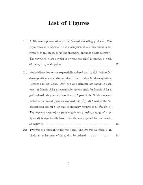
Page 5 and 6: 2.5 Nested dissection ordering . .
Page 7: 6.1.4 Waveeld inversion . . . . . .
Page 11 and 12: 4.3 Two representative source gathe
Page 13 and 14: 4.15 Frequency domain modelled (pre
Page 15 and 16: 5.3 Numerical dispersion of the new
Page 17 and 18: Chapter 1 Introduction Modelling th
Page 19 and 20: Pratt (1995) and Song (1995) showed
Page 21 and 22: parameters is a daunting task. Extr
Page 23 and 24: element methods. 1.2 The signicance
Page 25 and 26: this sparsity. As in time domain me
Page 27 and 28: where the complex \impedance" matri
Page 29 and 30: 1.4 Fourier transforms and frequenc
Page 31 and 32: in order to unambiguously reconstru
Page 33 and 34: If the forward Fourier transform is
Page 35 and 36: ased on data setfrom an underground
Page 37 and 38: therefore one of the main applicati
Page 39 and 40: 2.3 Solving linear equation systems
Page 41 and 42: are always calculated by the time t
Page 43 and 44: Case 2 2 S = ~ 6 4 4 0 0 0 .5 0 .79
Page 45 and 46: Figure 2.2: Two-way dissected nite
Page 47 and 48: (n/2*n/2)/2 L 55 (n/2*n/2)/2 n*n/2
Page 49 and 50: (to within anorder of magnitude) ne
Page 51 and 52: D 4 (n; 0) (2n) 2 =2 + 2(2n=2) 2 =
Page 53 and 54: The memory required to perform LU d
Page 55 and 56: are of theorder of hundereds of kil
Page 57 and 58: 10000 1000 Time (s) Sequential orde
Page 59 and 60:
Chapter 3 Visco-acoustic frequency
Page 61 and 62:
Figure 3.1: Finite dierence operato
Page 63 and 64:
However, analytical solutions do no
Page 65 and 66:
3.2.4 Lumped and consistent matrix
Page 67 and 68:
+4c=1 (3.9) which makes the minimiz
Page 69 and 70:
that the required memory is afuncti
Page 71 and 72:
1996). However quantitativeevaluati
Page 73 and 74:
(1991). The low velocity regions (1
Page 75 and 76:
a) Time slice at 5s b) Time slice a
Page 77 and 78:
domain approach would have to gener
Page 79 and 80:
1988). Reviews have been provided b
Page 81 and 82:
Figure 4.1: Grimsel Pass areal phot
Page 83 and 84:
5 10 15 20 25 30 35 40 45 50 55 60
Page 85 and 86:
160m BOUS 85.003 BOBK 85.004 BOBK 8
Page 87 and 88:
will assume that rst n r n x n z (
Page 89 and 90:
where jxj represents represents the
Page 91 and 92:
or c J~ = S ~ ,1 G ~ (4.13) where F
Page 93 and 94:
Figure 4.6: Comparison of the trave
Page 95 and 96:
In order to initialize the waveeld
Page 97 and 98:
the trace-to-trace amplitude variat
Page 99 and 100:
manner these groups were identied.
Page 101 and 102:
km/s 4.80 4.85 4.90 4.95 5.00 5.05
Page 103 and 104:
4.6.2 Regularization tests From thi
Page 105 and 106:
RMS Roughness 0.8 0.7 0.6 0.5 5 10
Page 107 and 108:
Figure 4.15: Frequency domain model
Page 109 and 110:
y the best isotropic results. In al
Page 111 and 112:
a) b) c) Figure 4.19: Data residual
Page 113 and 114:
Figure 4.20: Anisotropic full wavee
Page 115 and 116:
km/s 4.80 4.85 4.90 4.95 5.00 5.05
Page 117 and 118:
Figure 4.24: Final waveeld inversio
Page 119 and 120:
can eect theimages (the wrong theor
Page 121 and 122:
In essence, our new scheme is the e
Page 123 and 124:
where ! = 2f is the angular frequen
Page 125 and 126:
dicult to formulate direct solvers
Page 127 and 128:
! 2 u 0 + v 0 + ( +2) + ( + ) @ u
Page 129 and 130:
\stars": ! @ 2 1 0 0 1 0 -2 0 @x 0
Page 131 and 132:
free to vary from one node point to
Page 133 and 134:
(see equations 5.24 and 5.25), exce
Page 135 and 136:
1 1 0.8 0.8 a 0.6 0.4 b 0.6 0.4 0.2
Page 137 and 138:
Numerical dispersion curves for σ=
Page 139 and 140:
Ifollow closely the dispersion anal
Page 141 and 142:
the opposite results. The fraction
Page 143 and 144:
identied; it is also possible to id
Page 145 and 146:
Real data Acoustic modelling result
Page 147 and 148:
observed data. However, even with t
Page 149 and 150:
Chapter 6 Conclusions and further w
Page 151 and 152:
compensated for by the accuracy gai
Page 153 and 154:
(1992)). I have also shown how sens
Page 155 and 156:
Extensions to more complex cases Th
Page 157 and 158:
Although waveeld inversions have be
Page 159 and 160:
to nd more dicult targets. An incre
Page 161 and 162:
Bathe, K. J., and Wilson, E. L., 19
Page 163 and 164:
Cole, J. B., 1994, A nearly exact s
Page 165 and 166:
Lailly, P., 1984, Migration methods
Page 167 and 168:
Peng, C., Cheng, C. H., and Toksoz,
Page 169 and 170:
Smith, W. D., 1974, The application
Page 171 and 172:
Appendix A Dispersion analysis for
Page 173:
and 2 = ( 1 R 2 + 2 )( 1 + 2 R 2
show all

Frequency domain seismic forward modelling: A tool for waveform ...

Create successful ePaper yourself

Delete template?

Save as template?