Quantitative Description of Surface Structure
Quantitative Description of Surface Structure
Quantitative Description of Surface Structure

Create successful ePaper yourself
Turn your PDF publications into a flip-book with our unique Google optimized e-Paper software.
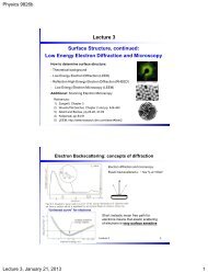
Physics 9826b_Winter 2013<br />
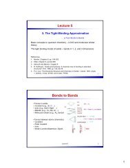
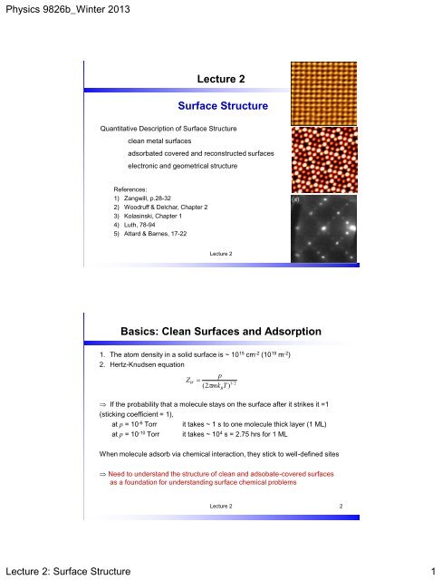
Lecture 2<br />
<strong>Surface</strong> <strong>Structure</strong><br />
<strong>Quantitative</strong> <strong>Description</strong> <strong>of</strong> <strong>Surface</strong> <strong>Structure</strong><br />
clean metal surfaces<br />
adsorbated covered and reconstructed surfaces<br />
electronic and geometrical structure<br />
References:<br />
1) Zangwill, p.28-32<br />
2) Woodruff & Delchar, Chapter 2<br />
3) Kolasinski, Chapter 1<br />
4) Luth, 78-94<br />
5) Attard & Barnes, 17-22<br />
Lecture 2 1<br />
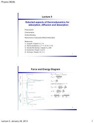
Basics: Clean <strong>Surface</strong>s and Adsorption<br />
1. The atom density in a solid surface is ~ 10 15 cm -2 (10 19 m -2 )<br />
2. Hertz-Knudsen equation<br />
Z<br />
W<br />
p<br />
<br />
( 2mk<br />
T)<br />
If the probability that a molecule stays on the surface after it strikes it =1<br />
(sticking coefficient = 1),<br />
at p = 10 -6 Torr it takes ~ 1 s to one molecule thick layer (1 ML)<br />
at p = 10 -10 Torr it takes ~ 10 4 s = 2.75 hrs for 1 ML<br />
B<br />
1/ 2<br />
When molecule adsorb via chemical interaction, they stick to well-defined sites<br />
Need to understand the structure <strong>of</strong> clean and adsobate-covered surfaces<br />
as a foundation for understanding surface chemical problems<br />
Lecture 2 2<br />
Lecture 2: <strong>Surface</strong> <strong>Structure</strong> 1
Physics 9826b_Winter 2013<br />
2.1 Bulk Truncation <strong>Structure</strong><br />
Ideal flat surface: truncating the bulk structure <strong>of</strong> a perfect crystal<br />
Miller Indices, revisited<br />
- For plane with intersections at b x , b y b z<br />
<br />
write reciprocals: <br />
1 1 1<br />
<br />
bx<br />
by<br />
bZ<br />
<br />
- If all quotients are rational integers or 0, this is Miller index<br />
e.g., b x , b y , b z = 1, 1, 0.5 (112)<br />
b x , b y , b z = 1, , (100)<br />
- In general<br />
cd<br />
Miller index ( i , j,<br />
k)<br />
<br />
bx<br />
e.g.,<br />
cd<br />
b<br />
y<br />
cd <br />
,<br />
b<br />
z <br />
12<br />
12 12 <br />
cd 12;<br />
( i,<br />
j,<br />
k)<br />
(643)<br />
2 3 4 <br />
where cd - common denom. <strong>of</strong><br />
b ,b ,b<br />
x<br />
y<br />
z<br />
Lecture 2 3<br />
x<br />
x<br />
b x<br />
b z<br />
2<br />
4<br />
z<br />
z<br />
3<br />
b y<br />
y<br />
y<br />
Crystallographic planes<br />
• Single plane (h k l)<br />
• Notation: planes <strong>of</strong> a family {h k l}<br />
(100); (010); (001); … {100} are all equivalent<br />
• Only for cubic systems: the direction indices <strong>of</strong> a direction<br />
perpendicular to a crystal plane have the same Miller indices as a<br />
plane<br />
• Interplanar spacing d hkl :<br />
d hkl<br />
<br />
h<br />
2<br />
a<br />
k<br />
2<br />
l<br />
2<br />
Lecture 2 4<br />
Lecture 2: <strong>Surface</strong> <strong>Structure</strong> 2
Physics 9826b_Winter 2013<br />
Metallic crystal structures (will talk about metal oxides later)<br />
• >90% <strong>of</strong> elemental metals crystallize upon solidification into 3 densely<br />
packed crystal structures:<br />
Body-centered cubic<br />
(bcc)<br />
Face-centered cubic<br />
(fcc)<br />
Hexagonal closepacked<br />
(hcp)<br />
ex.: Fe, W, Cr<br />
ex.: Cu, Ag, Au<br />
ex.: Zr, Ti, Zn<br />
Very different surfaces!!!<br />
Lecture 2 5<br />
fcc crystallographic planes<br />
Cu (100)<br />
Lecture 2 6<br />
Lecture 2: <strong>Surface</strong> <strong>Structure</strong> 3
Physics 9826b_Winter 2013<br />
fcc crystallographic planes<br />
Cu (110)<br />
Anisotropy <strong>of</strong> properties in two directions<br />
Lecture 2 7<br />
fcc crystallographic planes<br />
Cu (111)<br />
3 fold symmetry<br />
Lecture 2 8<br />
Lecture 2: <strong>Surface</strong> <strong>Structure</strong> 4
Physics 9826b_Winter 2013<br />
Atomic Packing in Different Planes<br />
• bcc (100) (110) (111)<br />
close-packed<br />
• fcc (100) (110) (111)<br />
Very rough: fcc (210) and bcc(111)<br />
Lecture 2 9<br />
Bulk Truncated <strong>Structure</strong>s<br />
Lecture 2 10<br />
Lecture 2: <strong>Surface</strong> <strong>Structure</strong> 5
Physics 9826b_Winter 2013<br />
Cubic System<br />
(i j k) defines plane<br />
[i j k] is a vector to plane, defining direction<br />
Cross product <strong>of</strong> two vectors in a plane defines direction perpendicular to plane<br />
[i j k] = [l m n] [ o p q]<br />
[i j k]<br />
[l m n]<br />
Angle between two planes (directions):<br />
<br />
[ ijk ] [<br />
lmn]<br />
cos <br />
2 2 2 2 2 2<br />
i j k l m n<br />
e.g., for [111], [211]<br />
cos <br />
2 2<br />
1 1<br />
1<br />
2 11<br />
2<br />
2 2 2<br />
2 1<br />
1<br />
4<br />
19.47<br />
3 2<br />
o<br />
Lecture 2 11<br />
Planes in hexagonal close-packed (hcp)<br />
4 coordinate axes (a 1 , a 2 , a 3 , and c) <strong>of</strong> the hcp structure (instead <strong>of</strong> 3)<br />
Miller-Bravais indices - (h k i l) – based on 4 axes coordinate system<br />
a 1 , a 2 , and a 3 are 120 o apart: h k i<br />
c axis is 90 o : l<br />
3 indices (rarely used):<br />
h + k = - I<br />
(h k i l) (h k l)<br />
Lecture 2 12<br />
Lecture 2: <strong>Surface</strong> <strong>Structure</strong> 6
Physics 9826b_Winter 2013<br />
Basal and Prizm Planes<br />
Basal planes;<br />
a 1 = ; a 2 = ; a 3 = ; c = 1<br />
(0 0 0 1)<br />
Prizm planes: ABCD<br />
a 1 = +1; a 2 = ; a 3 = -1; c = <br />
(1 0 -1 0)<br />
Lecture 2 13<br />
Comparison <strong>of</strong> Crystal <strong>Structure</strong>s<br />
FCC and HCP metal crystal structures<br />
void a<br />
void b<br />
A<br />
B<br />
Bb<br />
• (111) planes <strong>of</strong> fcc have the same arrangement as (0001) plane <strong>of</strong> hcp crystal<br />
• 3D structures are not identical: stacking has to be considered<br />
Lecture 2 14<br />
Lecture 2: <strong>Surface</strong> <strong>Structure</strong> 7
Physics 9826b_Winter 2013<br />
FCC and HCP crystal structures<br />
void a<br />
void b<br />
A<br />
B<br />
C<br />
A<br />
B<br />
fcc<br />
B plane placed in a voids <strong>of</strong> plane A<br />
Next plane placed in a voids <strong>of</strong><br />
plane B, making a new C plane<br />
Stacking: ABCABC…<br />
hcp<br />
B plane placed in a voids <strong>of</strong> plane A<br />
Next plane placed in a voids <strong>of</strong> plane B,<br />
making a new A plane<br />
Stacking: ABAB…<br />
Lecture 2 15<br />
Diamond, Si and Ge surfaces<br />
(100)<br />
(110)<br />
(111)<br />
Lecture 2 16<br />
Lecture 2: <strong>Surface</strong> <strong>Structure</strong> 8
Physics 9826b_Winter 2013<br />
Beyond Metals: polar termination<br />
Zincblend structure<br />
Note that polar terminations are not<br />
equivalent for (100) and (111)<br />
ZnS (100)<br />
Zn<br />
S -s<br />
+s<br />
-s<br />
+s<br />
-s<br />
+s<br />
-s<br />
+s<br />
capacitor model<br />
ZnS (111)<br />
Lecture 2 17<br />
Stereographic Projections<br />
crystal<br />
Project<br />
normals<br />
onto<br />
planar<br />
surface<br />
Normals to<br />
planes<br />
Lecture 2 18<br />
from K.Kolasinski<br />
Lecture 2: <strong>Surface</strong> <strong>Structure</strong> 9
Physics 9826b_Winter 2013<br />
2.2 Relaxations and Reconstructions<br />
Often surface termination is not bulk-like<br />
There are atom shifts or ║ to surface<br />
These surface region extends several atom layer deep<br />
Rationale for metals: Smoluchowski smoothing <strong>of</strong> surface electron charge;<br />
dipole formation<br />
Lecture 2 19<br />
Reconstructions<br />
Rationale for semiconductors: heal “dangling bonds<br />
<strong>of</strong>ten lateral motion<br />
Lecture 2 20<br />
Lecture 2: <strong>Surface</strong> <strong>Structure</strong> 10
Physics 9826b_Winter 2013<br />
2.3 Classification <strong>of</strong> 2D periodic <strong>Structure</strong>s<br />
Unit cell: a convenient repeating unit <strong>of</strong> a crystal lattice; the axial lengths and<br />
axial angles are the lattice constants <strong>of</strong> the unit cell<br />
Wigner –<br />
Seitz cell<br />
Larger than<br />
needed<br />
Unit cell is<br />
not unique!<br />
Wigner – Seitz Cell : place the symmetry centre in<br />
the centre <strong>of</strong> the cell; draw the perpendicular<br />
bisector planes <strong>of</strong> the translation vectors from the<br />
chosen centre to the nearest equivalent lattice site<br />
Lecture 2 21<br />
2D Periodic <strong>Structure</strong>s<br />
<br />
T na m<br />
Propagate lattice: n, m – integers<br />
Primitive unit cell: generally, smallest area, shortest lattice vectors, small<br />
number <strong>of</strong> atoms ( if possible |a 1 |=|a 2 |, a=60 o , 90 o , 120 o , 1 atom/per cell)<br />
1<br />
a 2<br />
Symmetry:<br />
- translational symmetry || to surface<br />
- rotational symmetry 1(trivial), 2, 3, 4, 6<br />
- mirror planes<br />
- glide planes<br />
All 2D structures<br />
w/1atom/unit cell have at<br />
least one two-fold axis<br />
Lecture 2 22<br />
Lecture 2: <strong>Surface</strong> <strong>Structure</strong> 11
Physics 9826b_Winter 2013<br />
2.4 2D Substrate and <strong>Surface</strong> <strong>Structure</strong>s<br />
Considering all possibilities and redundancies for 2D periodic structures (e.g.,<br />
3-fold symmetry for g=60 o , 120 o , we get only 5 symmetrically different<br />
Bravais nets with 1 atom per unit cell<br />
When more than 1 atom/unit cell<br />
more complicated:<br />
- 5 Bravais lattices<br />
- 10 2D point symmetry group (cf. Woodruff)<br />
- 17 types <strong>of</strong> surface structures<br />
Substrate and Overlayer <strong>Structure</strong>s<br />
Suppose overlayer (or reconstructed surface layer) lattice different from<br />
substrate<br />
<br />
T<br />
<br />
T<br />
A<br />
B<br />
<br />
na1<br />
ma2<br />
<br />
nb mb<br />
1<br />
2<br />
Lecture 2 23<br />
2.5 Wood’s notation<br />
Simplest, most descriptive notation method (note: fails if a ≠ a’ or b i /a i irrational)<br />
p(22)<br />
b 1<br />
b 1<br />
a’<br />
b 2<br />
b 2<br />
a 1<br />
a 2<br />
a<br />
a 2<br />
Procedure:<br />
- Determine relative magnitude <strong>of</strong> a 1 , b 1 , and a 2 , b 2<br />
- Identify angle <strong>of</strong> rotation (here f = 0) Notation:<br />
c(2 2) or<br />
p(2 2) R45 o<br />
b b <br />
1 2<br />
<br />
Rf<br />
a a<br />
1 2 <br />
Lecture 2 24<br />
Lecture 2: <strong>Surface</strong> <strong>Structure</strong> 12
Physics 9826b_Winter 2013<br />
2.6 Matrix Notation<br />
Use matrix to transform substrate basis vectors, a 1 , a 2 , into overlayer basis<br />
vectors, b 1 , b 2<br />
Lecture 2 26<br />
Lecture 2 25<br />
2.7 Comparison <strong>of</strong> Wood’s and Matrix Notation<br />
Classification <strong>of</strong> lattices:<br />
Lecture 2: <strong>Surface</strong> <strong>Structure</strong> 13
Physics 9826b_Winter 2013<br />
Examples <strong>of</strong> Coincidence Lattice<br />
Note that symmetry does not<br />
identify adsorption sites, only<br />
how many there are<br />
Domain structures:<br />
(1 X 2) = (2 X 1)<br />
Lecture 2 27<br />
Domains and domain walls<br />
heavy<br />
wall<br />
light<br />
wall<br />
Lecture 2 28<br />
Lecture 2: <strong>Surface</strong> <strong>Structure</strong> 14
Physics 9826b_Winter 2013<br />
Consider that in the pictures you are looking down at a surface. The larger circles<br />
represent the substrate atom positions and dark dots represent the overlayer atom<br />
positions. Overlayer unit cells are shown. For each structure:<br />
(1) Draw the substrate unit cell and vectors, and the primitive overlayer unit cell and unit<br />
cell vectors.<br />
(2) Calculate the ideal coverage (in monolayers) <strong>of</strong> the overlayer.<br />
(3) If the primitive overlayer surface unit cell can be named with Wood’s notation, do so.<br />
If it cannot, try to identify a nonprimitive cell which can be so named.<br />
(4) Give the matrix notation for the primitive overlayer unit cell.<br />
(5) Classify the surface overlayer as simple, coincident or incoherent.<br />
(a)<br />
29<br />
(b)<br />
Lecture 2 30<br />
Lecture 2: <strong>Surface</strong> <strong>Structure</strong> 15
Physics 9826b_Winter 2013<br />
Try (c) and (d) at home<br />
(c)<br />
Lecture 2 31<br />
(d)<br />
Lecture 2 32<br />
Lecture 2: <strong>Surface</strong> <strong>Structure</strong> 16