An acoustic Doppler velocimeter (ADV) for the ... - LTHE

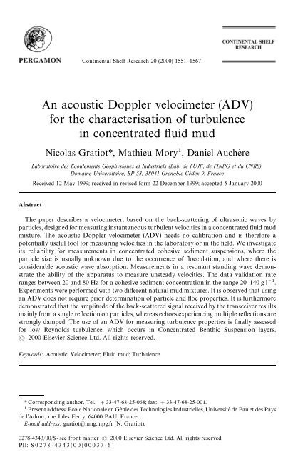
Continental Shelf Research 20 (2000) 1551}1567 

An acoustic Doppler velocimeter (ADV) 

for the characterisation of turbulence 

in concentrated #uid mud 

Nicolas Gratiot*, Mathieu Mory, Daniel Auchère 

Laboratoire des Ecoulements Ge& ophysiques et Industriels (Lab. de l'UJF, de l'INPG et du CNRS), 

Domaine Universitaire, BP 53, 38041 Grenoble Ce& dex 9, France 

Received 12 May 1999; received in revised form 22 December 1999; accepted 5 January 2000 

Abstract 

The paper describes a velocimeter, based on the back-scattering of ultrasonic waves by 

particles, designed for measuring instantaneous turbulent velocities in a concentrated #uid mud 

mixture. The acoustic Doppler velocimeter (ADV) needs no calibration and is therefore a 

potentially useful tool for measuring velocities in the laboratory or in the "eld. We investigate 

its reliability for measurements in concentrated cohesive sediment suspensions, where the 

particle size is usually unknown due to the occurrence of #occulation, and where there is 

considerable acoustic wave absorption. Measurements in a resonant standing wave demonstrate 

the ability of the apparatus to measure unsteady velocities. The data validation rate 

ranges between 20 and 80 Hz for a cohesive sediment concentration in the range 20}140 g l. 

Experiments were performed with two di!erent natural mud mixtures. It is observed that using 

an ADV does not require prior determination of particle and #oc properties. It is furthermore 

demonstrated that the amplitude of the back-scattered signal received by the transceiver results 

mainly from a single re#ection on particles, whereas echoes experiencing multiple re#ections are 

strongly damped. The use of an ADV for measuring turbulence properties is "nally assessed 

for low Reynolds turbulence, which occurs in Concentrated Benthic Suspension layers. 

2000 Elsevier Science Ltd. All rights reserved. 

Keywords: Acoustic; Velocimeter; Fluid mud; Turbulence 

* Corresponding author. Tel.: #33-47-68-25-068; fax: #33-47-68-25-001. 

Present address: Ecole Nationale en GeH nie des Technologies Industrielles, UniversiteH de Pau et des Pays 

de l'Adour, rue Jules Ferry, 64000 PAU, France. 

E-mail address: gratiot@hmg.inpg.fr (N. Gratiot). 

0278-4343/00/$ - see front matter 2000 Elsevier Science Ltd. All rights reserved. 

PII: S 0 2 7 8 - 4 3 4 3 ( 0 0 ) 0 0 0 3 7 - 6

1552 N. Gratiot et al. / Continental Shelf Research 20 (2000) 1551}1567 

1. Introduction 

During the few last decades, investigations in estuarine and coastal areas have 

shown the occurrence of near-bed layers in which concentrations of up to 200 g l 

can be measured. These #uid mud layers, also called concentrated benthic suspensions 

(CBS), are separated by a sharp interface (lutocline) from the upper water layer where 

the sediment suspension is dilute (Mehta, 1989). Several studies (Odd et al., 1993) have 

pointed out the importance of CBS for cohesive sediment transport. However, only 

a few surveys provide "eld observations of the CBS layer including suspended 

sediment concentration and velocity measurements (Trowbridge and Kineke, 1994). 

The di$culty in obtaining velocity measurements within the CBS layer stems from its 

thickness, which usually does not exceed a few centimetres, and the high concentration 

(20}200 g l). 

Various methods have been considered for measuring #ow velocity in natural 

sediment suspensions. Using a hot "lm probe led to failure resulting from particle 

impingement on the sensor (Fukuda and Lick, 1980). Laser Doppler anemometry 

does not operate in #uid mud because the incident laser beams are rapidly attenuated 

and the light di!used by the particles is spread when the sediment concentration 

exceeds a few hundred milligrams per litre (Baker and Lavelle, 1984). Micropropeller 

current meters are often used in "eld surveys, but they only provide an estimate of the 

mean current. Turbulent velocity measurements have been made using radioactive 

tracers (Berlamont, 1989), dyed material (Sakakiyama and Bijker, 1989), and electromagnetic 

current meters (Sternberg et al., 1991; de Witt and Kranenburg, 1996). The 

electromagnetic current meter has proved to be a useful tool in shallow water 

environments and in "eld deployments, but one of its limitations is due to its spatial 

resolution (van der Ham, 1999; Soulsby, 1980). 

Ultrasonic probes are an attractive technology for measuring unsteady velocities as 

they are non-intrusive remote sensing systems. Various systems have been developed, 

some of which allow the three velocity components to be measured simultaneously at 

a single point while others provide instantaneous measurements of velocity pro"les. 

Their application in assessing sediment #uxes in marine environments is di$cult 

because ultrasonic waves are absorbed in sediment-laden #ows. Instantaneous sediment 

#ux pro"les were nevertheless successfully measured in the laboratory with 

quartz-like particles having concentrations as high as 28 g l (Shen and Lemmin, 

1997). In the "eld, despite the heterogeneity of the natural material, acoustic backscattering 

has been used to measure the mean velocity in a tidal #ow (Lhermitte, 1983) 

and in an estuarine environment (Thorne et al., 1998). 

Most systems have been used up to now in sand-like sediment-laden #ows. This 

article considers the case of natural cohesive sediments having high concentration 

values (in the range 20}160 g l). This investigation was conducted in the course of a 

laboratory study of the occurrence and properties of CBS layers, for which it was 

desirable to measure turbulent unsteady velocities. The aim of the study presented in 

this paper was to examine the ability of an ADV system to measure instantaneous 

velocities in concentrated #uid mud. A standard ADV system was used, the principle 

of operation of which is based on analysis of the back-scattered phase change

N. Gratiot et al. / Continental Shelf Research 20 (2000) 1551}1567 1553 

observed from pulse to pulse. Because this apparatus was built in our laboratory, the 

settings could be conveniently modi"ed. Several di$culties have to be considered 

when applying ultrasonic methods in #uid mud. First of all, acoustic waves are subject 

to absorption and multiple scattering. Secondly, particle sizes may change as a result 

of #occulation in cohesive sediment suspensions. They are usually not known precisely. 

An attempt was made to determine whether an ADV can operate without prior 

determination of #oc size and whether the quality of operation depends on the 

composition of the mud. Because the apparatus is not new in itself, the operating 

principle is only brie#y described in Section 2. The focus in Section 3 is then on the 

reliability of this apparatus for measurements in cohesive sediment suspensions. 

Unsteady velocity measurements were performed in a standing wave #ow. They are 

presented in Section 4. The precision of measurement, rate of data acquisition, and 

quality of measurement as a function of sediment concentration were determined. 

Measurements in turbulent #ows were "nally carried out. The statistical properties of 

the turbulence measurements are presented in Section 5. 

2. Principle of operation of the ADV 

The ADV system is based on a Doppler Sonar concept described previously by 

Lhermitte (1983). The latter showed that such an apparatus is appropriate for 

measuring mean vertical pro"les of the longitudinal velocity in a tidal channel. Our 

application case is very di!erent as the aim here is to measure velocities in highly 

concentrated #uid mud, with su$cient spatial and temporal resolutions to measure 

turbulence. 

The ADV operating principle di!ers from more classical ADV systems which 

deduce the velocity from measurements of the Doppler frequency shift 2ω 

v/c of the 

re#ected signal, ω 

being the pulsation of the emitted pulse. Even if a long transmitter 

pulse is analysed, this method is not applicable for low velocities because determining 

the Doppler frequency using Fourier analysis is not very accurate. Analysing the 

back-scattered echoes in terms of changes in the time shift ¹ ( 

"2vt/c of pulse-topulse 

back-scattered signals, as done by our apparatus and described by Lhermitte 

(1983), provides a much better resolution of velocity. As the volume of measurement is 

not in"nitely small, the received signal is a combination of echoes back-scattered by a 

randomly distributed set of particles. The pulse-to-pulse Doppler system requires 

several successive echoes to remain coherent. This condition is satis"ed if the volume 

of measurement and the period of repetition ¹ 

between two successive pulses are 

su$ciently small to consider that the motion is approximately of solid body type 

inside the measurement volume. Furthermore the velocity must be constant over a 

period that covers a su$cient number of successive echoes. 

The speci"cations of the ADV, as shown in Fig. 1, were determined with regard to 

the previous conditions. In order to reduce the volume of measurement, the beam is 

convergent, focusing the sound wave in a focal zone F 

where the beam cross-section 

is almost constant. Its value is of the order of 1.5 mm, corresponding to the transverse 

distance where the wave energy is !6 dB the value of the wave energy on the axis of


Fig. 1. Transducer speci"cations: (a) Multigate pro"ling system; (b) Shape of the emitted pulse; (c) Size of 

measurement volume. 

the beam. Measurements are made in this section of length F 

"8.8 cm in front of the 

beam probe. The depth of the volume of measurement is dependent on the frequency 

f 

and the number of periods n 

of the emitted pulse. The value is presently of the 

order of 0.5 mm as f 

"5 MHz and n 

+3. This speci"cation gives a volume of 

measurement of nearly 1 mm. It may be noticed that the volume of measurement is 

smaller than those of classical electromagnetic current meters (a few cm) usually used 

to measure velocity in estuaries. An option of our system, by gating the back-scattered 

signal in "ve successive time windows, enables the velocities to be determined at "ve 

distances along the beam. 

The minimum value for the periodicity ¹ 

of wave packet emissions is determined 

by considering the position of measurement, because a back-scattered echo has to be 

received before sending the next pulse. During this study, pulse emission periods of 

¹ 

"0.128 ms and ¹ 

"0.256 ms were used. The corresponding maximum distances 

of measurement from the probe are c¹ 

/2+10 cm and c¹ 

/2+20 cm. There is also 

a maximum distance of measurement from the probe on account of the ultrasonic 

wave absorption properties of the sediment mixture (see Section 3). 

The time shift increase between two successive back-scattered echoes of two wave 

packets emitted at a time interval ¹ 

is 

¹ ( 

(i#1)!¹ ( 

(i)" 2v 

c ¹ . (1) 

Time shift values are digitised for successive wave packets and stored in a "le. As an 

example, a 29 ms record of the changes in time shift of the back-scattered echoes for 

226 successive wave packets is shown in Fig. 2. It displays a saw tooth behaviour as


Fig. 2. Typical record of changes in time shift versus time. The software validates the calculated velocity if 

the correlation between a minimum of n"10 data and a "tted straight line is su$cient. 

the phase of the back-scattered echo is between 0 and T . While the velocity can be 

 

deduced from Eq. (1), the velocity averaged over a time interval of duration N¹ is 

instead determined numerically by "tting a straight line to a minimum of n successive 

time shift data (N"50 and n"10 for the example in Fig. 2), in order to reduce the 

variability in measurements. Fitting a straight line to at least n successive time shift 

data requires that ¹ (i#n)!¹ (i) should be less than T . This condition "xes the 

( ( 

upper bound of the measurement velocity range, 

v((¹ /n¹ )(c/2)+12 cm s, (2) 

 

as derived from Eq. (1) for n"10 and T "0.128 ms. The estimated velocity is 

 

validated as being in su$ciently good correlation, as obtained for instance for the data 

contained in the "rst two saw teeth in Fig. 3. The third saw tooth displays more 

scatter; the estimated data cannot be validated when N¹ is too large as compared to 

 

the typical time scale of variation of the velocity. If we consider the vertical deviation 

ε of datas to the straight line, the velocity is validated as long as the standard deviation 

σ is lower than 0.06T (see Fig. 3). 

 

3. Limitations for using an ADV in concentrated 6uid mud mixtures 

Speci"c questions arise in relation to the use of an ADV in cohesive sediment 

mixtures. In the "eld, the size of cohesive sediment #ocs can change drastically within 

the #uid mud because of the steep velocity gradients and because of the changes in 

concentration. Acoustic systems have already been used in cohesive sediment suspensions 

(Land et al., 1997). The e$ciency of back-scattering is linked to the nature of the 

sediments. The intensity and propagation of an acoustic wave packet is a!ected by


Fig. 3. Output voltage of the back-scattered echo received at time t after emission of a wave packet. 

d 

"ct/2 is the position of the back-scattering if only a single re#ection occurs. Grey line: no sediment in the 

domain 0(d 

(5 cm. Dark line: #uid mud mixture in the domain 0(d 

(5 cm; 4a) C"70 g l, 4b) 

C"194 g l.The zero-mean voltage has been o!set to improve readability. 

absorption, scattering by suspended particles, or by the presence of gas bubbles. 

Furthermore, it can change drastically, depending on the size and shape of the 

particles (Richards et al., 1996). For the purpose of experimental studies with natural 

mud mixtures, where the #oc properties are not known, we checked whether accurate 

velocity measurements required prior knowledge of #oc properties. 

Absorption and multiple re#ections of acoustic waves are two processes that have 

to be considered for using ultrasonic methods within #uid mud mixtures. On the one 

hand, the increase in ultrasonic wave absorption with increasing mud concentration 

implies a reduction in the magnitude of the back-scattered signals. This process sets 

a bound to the maximum distance of velocity measurement but it does not appear by 

itself to preclude using an ADV in a concentrated #uid mud mixture. On the other


hand, it is very important to quantify the contribution of the echoes received after 

multiple re#ections in the magnitude of the back-scattered signal, since the ADV 

operating principle assumes a single re#ection for each echo analysed. 

Experiments were conducted in a small tank to assess the occurrence of single or 

multiple re#ections and to quantify absorption. The tank contained two chambers (A 

and B, respectively) separated by a thin "lm of plastic. Chamber A was "lled with #uid 

mud mixture while chamber B contained clear water. The probe was plunged into 

A and emitted a single pulse in the direction of B. Back-scattered acoustic echoes were 

recorded versus time. Fig. 3 presents the variation versus time in the magnitude of 

echoes produced in #uid mud mixtures at two di!erent concentrations (70 and 

194 g l). To interpret the diagrams, d 

"ct/2 is used instead of time; it is the distance 

from the probe where the echo received at time t was back-scattered if a single 

re#ection occurred. The acoustic propagation celerity is assumed to be constant and 

uniform in A and B (c"1500 m s). We will show later that this condition is 

validated. As the probe is acting both as emitter and receiver, the emission of acoustic 

wave packets considerably disturbs the piezoelectric sensor; measurements are not 

available for a short time after emission, which corresponds to a distance of approximately 

5 mm. When the two chambers contain clear water, back-scattering is insigni"cant 

in the domains 5 mm(x(48 mm and x'52 mm (parts A and B of the tank, 

respectively), as the absence of scatterers hinders re#ection. An echo of small amplitude 

is, however, observed at a distance of 50 mm. This is the re#ection of the acoustic 

pulse on the thin plastic "lm separating the two chambers. When sediments are 

contained in section A, we can quantify the relative importance of multiple re#ection 

echoes in the amplitude of the received signal by comparing the magnitude of echoes 

for x'50 mm and x(50 mm (dark plots) in Fig. 3. If a signi"cant proportion of the 

echoes is related to multiple re#ection events, the magnitude of the signal should be 

comparable on both sides of x"50 mm. Actually, the magnitude of echoes for 

x'50 mm is as low as it is when measured in clear water (gray lines in Fig. 3), where 

no sediment is present. The graphs in Fig. 3 do not indicate that multiple re#ections 

are not occurring, but that there is considerable absorption of acoustic waves when 

multiple re#ections do occur. The magnitude of echoes resulting from multiple 

re#ections is as low as the magnitude of echoes in clear water, and the magnitude of 

echoes resulting from a single re#ection predominates in the back-scattered signal. 

For a low sediment concentration (Fig. 3(a)), the received output voltage of echoes is 

high and has an almost constant amplitude for x(50 mm. In that case, the absorption 

is small and the magnitude of the acoustic pulse is not a!ected by sediment loading. 

The distance for which the amplitude of the signal drops corresponds to the distance 

of the plastic "lm. It is exactly the distance of the echo when the two chambers contain 

clear water. This indicates that the acoustic propagation celerity is constant. For 

a higher sediment concentration (Fig. 3(b)) the magnitude of the echoes decreases 

rapidly in front of the probe. For the highest concentration considered (194 g l), 

echoes are no longer detected at more than 35 mm from the probe. 

To identify the e!ects of mud properties on ADV measurements, experiments were 

performed using two di!erent natural muds, extracted from the Gironde estuary 

(France) and from the Tamar estuary (UK). The mineralogical compositions of


Table 1 

Mineral composition of mud in the Tamar and Gironde 

Gironde Tamar 

D in μm 

12 15.0 

Grain size distribution sand (63}100 μm) 3 7.8 

(% by weight) mud ((63 μm) 97 92.2 

Gironde mud and Tamar mud were determined by de Croutte et al. (1996) and Feates 

et al. (1999), respectively. They are given in Table 1. Gironde mud contains about 30% 

of quartz. As quartz is known to be a good ultrasonic re#ecting surface, the presence 

of a signi"cant quantity of quartz suggests there should be a good ADV response. 

While Gironde mud was chemically treated with potassium permanganate and passed 

through a 100 μm sieve, Tamar mud was neither treated nor sieved. The ADV system 

was used in di!erent mixtures with sediment concentrations in the range 20}160 g l. 

The mud properties (in particular for Tamar mud) in the tank were representative of 

those occurring in the "eld. For the high concentrations considered, it is to be 

expected that "ne sediments and #ocs are both present in the measurement volume. 

4. Unsteady velocity measurements in a concentrated 6uid-mud mixture 

The accuracy of measurements was determined for 10 di!erent mixtures with 

sediment concentrations of up to 160 g l. Velocity measurements were carried out 

in a resonant standing wave within a tank of "nite length (Fig. 4). Furthermore, in this 

unsteady #ow, it is possible to quantify the ability of the ADV to make unsteady #ow 

measurements, by determining the data measurement rate. In the linear regime, 

a simple theory relates free surface motions to the velocity "eld in the water layer. The 

accuracy of the ADV was estimated by comparing velocity measurements to the 

theoretical estimates of velocity variations deduced from measurements of free surface 

motions, as no other technique was available for comparing velocity measurements 

among themselves. 

Fig. 4 shows a sketch of the experimental set-up, consisting of a small #ume of 

length ¸"25.0 cm and width 9.0 cm. The water depth was set to h"5.0 cm. Gravity 

waves were generated mechanically by oscillating a vertical plate located in the middle 

of the #ume with the period of oscillation of resonant standing waves 

¹"2 π¸ 

g tanh(πh/¸) , (3) 

where g denotes the acceleration due to gravity. The plate was removed when surface 

waves were established and their amplitude appeared to be qualitatively constant. 

After approximately 10 s, secondary modes were dissipated and the resonant wave 

mode was then predominant. The oscillation amplitude decreased slowly due to


Fig. 4. Resonant gravity wave facility. Free surface oscillations are measured using an ultrasonic wave 

gauge. The ADV is immersed in a separate chamber. 

Fig. 5. Time-dependent changes in free surface displacements for a resonant standing wave: () experimental 

data, (*) model function given by Eq. (4). 

bottom and side-wall friction. The time record of the free surface displacements 

measured using an ultrasonic wave gauge at a "xed location in the #ume is shown in 

Fig. 5. The time-dependent changes in free surface motions were in good agreement 

with a function of the form 

η(x, t)"a e cos(πx/¸) cos(ωt) (4) 

 

(ω"2π/¹), which is superimposed on the data. This indicates that the wave energy is 

entirely contained in the resonant standing wave mode. Exponential decay accounts 

for viscous dissipation. While the wave frequency was determined theoretically, the 

initial amplitude a and the wave decay rate α were estimated from the free surface 

 

displacement record for each condition investigated. 

The transducer was placed in a section of the tank separated by a Plexiglas wall 

from the part of the tank where the gravity wave #ow was generated (see Fig. 4). The


section where the transducer was located was "lled with tap water, to ensure the 

propagation of acoustic waves through the Plexiglas wall between the probe and the 

position of measurement. Any #ow disturbance due to the ADV probe was therefore 

eliminated. Just before generating the gravity wave, the #uid mud mixture was fully 

mixed by hand. Obviously, the sediment settles slowly when mechanical mixing is 

stopped. The interface separating #uid mud and clear water was clearly visible in our 

experiments. The slow downward displacement of the interface provided an estimate 

of the settling velocity w 

. The latter quantity was found to be less than 1 mm s 

(generally 0.3 mm s). We therefore estimate that the concentration at the position of 

velocity measurement did not drop below the mean concentration before 

t'h 

/w 

+40s (h 

is the water depth above the measurement volume; the position of 

measurement was located 1 cm above the bottom). The velocity was measured during 

the time interval 20 s(t(30 s after the gravity wave was generated. The wave height 

remained of su$cient magnitude during this time interval. The variation in mud 

concentration with time, if it occurred, must have increased as a consequence of 

settling. The averaged mud concentration was measured from bottle samples taken 

from the initial #uid mud mixture. 

For the free surface displacements given by Eq. (4) the variation in the horizontal 

velocity component predicted by the linear potential theory is 

u(x, z, t)"! a gk 

ω 

cosh k(z#h) 

e sin(kx) sin(ωt), (5) 

cosh kh 

where h is the mean depth of the water layer inside the tank, z is the vertical 

co-ordinate (here at the position of measurement) and z"!h is on the bottom. 

Solution (5) veri"es u(0, t)"u(¸, t)"0 on the boundaries of the tank. 

Free surface and velocity measurements were not actually performed simultaneously 

in order to avoid any disturbance of the #ow by the wave gauges immersed in 

the tank. Considering Eq. (5), a function of the form 

u (x, z, t)"u 

e sin(ωt#θ), (6) 

was superimposed on the experimental data after adjusting the initial amplitude 

u 

and phase θ, while the wave height decay rate α was determined from the wave 

gauge records. 

Fig. 6 shows the time records of the velocity measured for three sediment concentrations 

(43, 50 and 100 g l) of Gironde or Tamar mud. The best agreement between 

the experimental data and Eq. (6) is observed for the lowest concentrations, i.e. C"43 

and C"50 g l. For the higher concentration C"100 g l, a few signi"cant errors 

arise when the velocity is maximum, but wave motion and wave decay are satisfactorily 

accounted for in the experimental data records. We believe that the variations at 

maximum velocity are measurement errors rather than turbulence production, because 

they are mainly observed for the higher concentration. Turbulence resulting 

from internal wave breaking is less likely to occur for the higher concentration. Each 

record displays short time intervals containing no data; these correspond to periods 

during which the software did not validate the velocity measurements. The data


Fig. 6. Horizontal velocity measurement in a resonant standing wave #ow. Gironde mud is used for the 

plots in (a) and (b). Tamar mud is used for the plot in (c). (a) C"100 g l, (b) C"50 g l, (c) C"43 g l. 

(, , ): ADV measurements, (*) model.


Fig. 7. Isoline of the rate of validation of velocity measurements (data per second) versus suspended 

sediment concentration C and versus distance of measurement from the sensor d 

. 

records display slight asymmetries, which are not understood. The wave model used 

for comparison is linear and does not include secondary-mode oscillations. Although 

the observed asymmetry is not signi"cant, it is surprising that the asymmetry in Figs. 

6(a) and (b) is opposite in direction to that in (c). No di!erence was observed in the 

accuracy of the measurements and in the rate of measurement between the Gironde 

and Tamar mud mixtures. Fig. 7 quanti"es the variations in measurement validation 

rate. The isoline plots were interpolated from a set of 60 cases for di!erent distances of 

measurement d 

from the probe and for di!erent concentrations of Tamar #uid mud 

mixtures. The maximum validation data rate is 78.1 Hz as ¹ 

"0.256 ms (N"50). As 

expected, the rate of data validation increases for decreasing concentration and 

decreasing distance of measurement from the probe. It is therefore established that the 

ADV system can measure unsteady velocities in #uid mud mixtures with concentrations 

of up to 140 g l with a data validation rate better than 20 data s. 

5. Measurements of turbulent velocity in a concentrated 6uid mud mixture 

The determination of turbulent velocities in #uid mud layers is a necessary step for 

assessing the vertical transfer of sediments between the muddy bed and the dilute 

suspension in estuarine environments. The investigations described in Section 4 demonstrated 

the ability of an ADV to make accurate measurements of unsteady velocities 

in concentrated #uid mud mixtures. The rate of validation, in the range 20}75 

data s, is not high, but it may be su$cient for turbulence measurements in 

concentrated Benthic suspensions in the "eld, where the velocity is quite low. A limitation 

on using an ADV for turbulence measurements in concentrated #uid mud


mixtures is the size of the measurement volume. For our system, this is typically 

0.5 mm in the direction of propagation of ultrasonic waves and 1.5 mm in the 

perpendicular direction (see Section 2). The ADV operates on the principle that 

solid-body motion is achieved inside the measurement volume. The size of the 

measurement volume must therefore be smaller than the smallest scale of turbulence. 

In order to investigate the ability of the ADV to measure turbulence properties, 

turbulence velocity variations were recorded in a simple sediment mixing experiment 

and some of the statistical properties of the turbulence were determined. 

The sediment was mixed in a square tank, 0.3 m wide and 0.2 m deep, by a rapidly 

rotating propeller. The propeller was set to a su$ciently rapid speed to maintain all 

the sediment in suspension. Velocity measurements were made in #uid mud mixtures 

of various concentrations (20, 50, 80 and 100 g l). Before the velocity was measured, 

the water and sediment were mixed for about 10 min and visual observations were 

made through the transparent bottom of the tank to ensure that no sediment 

remained deposited there. 

Fig. 8. presents a time history record measured by the ADV, covering a period of 

128 s. Each velocity datum was determined from the changes in phase shift averaged 

over a set of N"50 successive wave packets. For this experiment, the period of wave 

packet emission was decreased to T 

"0.128 ms, allowing a rate of measurement of 

156.2 Hz if all velocity data were validated. Actually, about 30% of the data were 

rejected and the record contains about 14,000 validated velocity data. For further 

Fig. 8. Velocity record measured by ADV in a mixing tank containing #uid mud of concentration 

C"50 g l.


Fig. 9. Distribution of a velocity record (plotted in Fig. 8) measured in a mixing tank containing #uid mud. 

A Gaussian distribution (*) is superimposed. 

analysis, the missing values in the record were replaced with the last preceding 

validated velocity datum. The propeller generated both a mean rotating #ow and 

turbulence. For this record, the mean velocity in the direction of propagation of 

ultrasonic waves is ;M "1.25 cm s and the rms turbulent velocity is u"2.15 

cm s. The histogram of velocity variations for the record considered in Fig. 8. is 

shown in Fig. 9. The distribution is Gaussian, as shown by the Gaussian curve 

superimposed on the data. This is a "rst indication that the statistical properties of the 

turbulence are captured in the velocity records measured by the ADV. As random 

white noise also displays a Gaussian distribution of events, a time frequency spectral 

analysis of velocity records was made in order to estimate the proportion of the signal 

corresponding to turbulent #ow and that associated with noise. The power spectrum 

of turbulent #uctuations is presented in Fig. 10. Energy density decays as frequency 

increases. The threshold level reached at frequencies higher than 70 Hz indicates the 

level of noise contained in the record. In hydrodynamic turbulent #ows, the energy 

density decays for increasing frequency, a phenomenon that is associated with a transfer 

of energy from low frequencies (large eddies) to high frequencies (small eddies). In 

Fig. 10, the energy spectrum decay versus frequency follows approximately a power 

law of the form E( f )+f , which is the decay law predicted by Kolmogorov's 

theory for a homogeneous isotropic turbulent #ow. Although these observations do 

not prove that the turbulence measurements are quantitatively accurate, they provide 

consistent indications that ADV measurements capture the hydrodynamic properties 

of turbulence and, in particular, that aliasing due to an insu$cient rate of data 

validation is unlikely to occur.


Fig. 10. Power spectrum of turbulent #ow velocity measured by the ADV in a mixing tank containing #uid 

mud. Suspended sediment concentration is C"100 g l. 

The integral length scale l of turbulence was not measured, and, therefore, only 

a range of variations of the Taylor microscale λ 

"l(ul/ν) can be inferred. The 

Taylor microscale varies in the range 0.7}7 mm for a rms turbulence velocity in the 

range 1}10 cm s and an integral length scale in the range 1}10 cm (ν" 

510 cm s for this estimate). The Taylor scale of turbulence is seen to be larger 

or, in some cases, may be of the order of the size of the measurement volume. The 

measurement volume of the ADV appears to be su$ciently small for the turbulence 

measurements carried out during the present investigation. 

6. Conclusions 

The present paper does not intend to present a new acoustic back-scatter system, 

but rather to investigate whether such a system can measure unsteady and turbulent 

velocities in concentrated #uid mud mixtures, and to determine the appropriate 

settings of the apparatus. For the purpose of making measurements in the laboratory, 

but also potentially in the "eld, di!erent natural muds were employed. An ADV does 

not require calibration and is a non-intrusive measurement device. It is therefore an 

attractive technology for measuring velocities in the laboratory and in the "eld. 

Speci"c questions arise concerning the use of an ADV in the presence of cohesive 

sediments. Acoustic wave absorption is enhanced in concentrated mud suspensions, 

but it does not hinder the reception of back-scattered echoes, even for concentrations 

as high as 100 g l, and when the distance of measurement from the probe is as far as 

50 mm. On the other hand, the considerable absorption of acoustic waves in their


interactions with particles appears to eliminate echoes resulting from multiple scattering 

in the back-scattered signal received by the transducer. A simple experiment was 

carried out, that shows that echoes resulting from multiple scattering make a negligible 

contribution to the signal received by the transducer in the time window 

considered for signal analysis. 

The accuracy of velocity measurements by an ADV has been demonstrated, 

without prior determination of particle and #oc sizes, in an unsteady laminar #ow, for 

sediment concentrations in the range 20}160 g l. Data rate validations were found 

to be in the range 20}75 for a rate of measurement of 78.1 Hz. While this is not a high 

rate of data acquisition, it is su$cient for many applications, especially in concentrated 

Benthic suspensions where velocities are not high. Turbulence measurements 

were carried out in a mixing tank containing a #uid mud mixture. By setting the 

period of pulse repetition to ¹ 

"0.128 ms we improved the rate of data acquisition 

up to 110 data s. The ADV measurement volume (0.5}1.5 mm) was smaller than the 

Taylor microscale of turbulence and the usual statistical behaviour of hydrodynamic 

turbulence was recovered by the ADV measurements made in the mixing tank. ADV 

appears to be an appropriate tool for measuring low Reynolds turbulence. 

Although this was not tested in the course of this study, using an ADV system for 

measuring velocities in #uid mud mixtures in the "eld is not a priori subject to any 

particular restriction, as far as the principle of operation is concerned. The principle of 

operation of our system is a standard one. Commercial pulse to pulse ADV systems 

should work as well, and sometimes may provide measurements of several velocity 

components. Using ADV is especially attractive because the measurement volume is 

small and it does not require calibration. For the present settings of our ADV system, 

the maximum velocity that can be measured is 12 cm s. It is certainly desirable to 

increase the range of measurements in order to use our ADV system in the "eld. Eq. (2) 

indicates the signi"cant settings of the apparatus. The period of pulse emission 

¹ 

cannot be reduced much as it "xes the location of measurement, which has to be 

su$ciently far from the probe. To increase the velocity range it would be necessary to 

increase the acoustic frequency f 

or to decrease the number n of echoes analysed for 

determining a velocity datum. The settings of the apparatus were f 

"5 MHz and 

n"10 in our study. The velocity range can presumably be increased, but checks 

should be made to determine how far the accuracy of measurements is reduced if the 

number n of data used for velocity determination is decreased. The ability of ADV for 

measurements in the "eld has to be evaluated. 

Acknowledgements 

This work was carried out as part of the COSINUS Program, which is funded 

by the European Commission (contract MAS3-CT97-0082). SogreH ah IngeH nierie is 

thanked for providing natural mud samples from the Gironde estuary. K. Dyer and 

A. Manning are thanked for providing natural mud samples from the Tamar estuary. 

K. Dyer is "nally thanked for having drawn our attention to the paper by Lhermitte 

(1983).


References 

Baker, E.T., Lavelle, W.J., 1984. The e!ect of particle size on the light attenuation coe$cient of natural 

suspensions. Journal of Geophysical Research 89 (C5), 8197}8203. 

Berlamont, J., 1989. Pumping #uid mud } theoretical and experimental considerations. In: Mehta, A.J., 

Hayter, E.J. (Eds.), High Concentration Cohesive Sediment Transport. Journal of Coastal Research 

(Special issue No. 5), 195}205. 

de Croutte, E., Gallissaires, J.M., Hamm, L., 1996. Flume measurements of mud processes over a #at 

bottom under steady and unsteady currents. SogreH ah IngeH nierie Report No. R3, December. 

de Wit, P., Kranenburg, C., 1996. On the e!ects of a lique"ed mud bed on wave and #ow characteristics. 

Journal of Hydraulic Research 34 (1), 3}18. 

Feates, N.G., Hall, J.R., Mitchener, H.J., Roberts, W., 1999. COSINUS "eld experiment, Tamar Estuary, 

measurement of properties of suspended sediment #ocs and bed properties. Report No. TR 82, HR 

Wallingford, March. 

Fukuda, K., Lick, W., 1980. The entrainment of cohesive sediments in freshwater. Journal of Geophysical 

Research 85 (C5), 2813}2824. 

Land, J.M., Kirby, R., Massey, J.B., 1997. Developments in the combined use of acoustic doppler current 

pro"lers and pro"ling siltmeters for suspended solids monitoring. In: Burt, N., Parker, R., Watts, J. 

(Eds.), Cohesive Sediments. Wiley, New York, pp. 187}196. 

Lhermitte, R., 1983. Doppler sonar observation of tidal #ow. Journal of Geophysical Research 88 (C1), 

725}742. 

Mehta, A.J., 1989. On estuarine cohesive sediment suspension behavior. Journal of Geophysical Research 

94 (C10), 14 303}14 314. 

Odd, N.V.M., Bentley, M.A., Waters, C.B., 1993. Observations and analysis of the movement of #uid mud in 

an estuary. In: Mehta, A.J. (Ed.), Nearshore and Estuarine Cohesive Sediment Transport, Coastal and 

Estuarine Studies, Vol. 42. AGU, Washington, DC, pp. 430}446. 

Richards, S.D., Heathershaw, A.D., Thorne, P.D., 1996. The e!ect of suspended particulate matter on sound 

attenuation in seawater. Journal of the Acoustical Society of America 100 (3), 1447}1450. 

Sakakiyama, T., Bijker, E.W., 1989. Mass transport velocity in mud layer due to progressive waves. Journal 

of Waterway, Port, Coastal and Ocean Engineering 115 (5), 614}633. 

Shen, C., Lemmin, U., 1997. A two-dimensional acoustic sediment #ux pro"ler. Measurement Science 

Technology 8, 880}884. 

Soulsby, R.L., 1980. Selecting record length and digitization rate for near bed turbulence measurements. 

Journal of Physical Oceanography 10, 208}219. 

Sternberg, R.W., Kineke, G.C., Johnson, R., 1991. An instrument system for pro"ling suspended sediment, 

#uid, and #ow conditions in shallow marine environments. Continental Shelf Research 11 (2), 109}122. 

Thorne, P.D., Hardcastle, P.J., Dolby, J.W., 1998. Investigation into the application of cross-correlation 

analysis on acoustic backscattered signals from suspended sediments to measure nearbed current 

pro"les. Continental Shelf Research 18, 695}714. 

Trowbridge, J.H., Kineke, G.C., 1994. Structure and dynamics of #uid muds on the Amazon continental 

shelf. Journal of Geophysical Research 99 (C1), 865}874. 

van der Ham, R., 1999, Turbulent exchange of "ne sediment in tidal #ow. Ph.D. Thesis, TUDelft.

An acoustic Doppler velocimeter (ADV) for the ... - LTHE

You also want an ePaper? Increase the reach of your titles

Delete template?

Save as template?