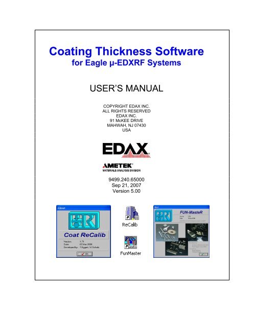
Coating Thickness Software for Eagle Âµ-EDXRF Systems

Coating Thickness Software 

for Eagle µ-EDXRF Systems 

USER’S MANUAL 

COPYRIGHT EDAX INC. 

ALL RIGHTS RESERVED 

EDAX INC. 

91 McKEE DRIVE 

MAHWAH, NJ 07430 

USA 

9499.240.65000 

Sep 21, 2007 

Version 5.00

1.1.2 ReCalib 2

Contents 

1. Introduction ................................................................................ 6 

1.1 The Software Packages .......................................................................................................................6 

1.1.1 FunMaster .................................................................................................................................6 

1.1.2 ReCalib......................................................................................................................................7 

1.2 SCATTER (excitation) SPECTRA ........................................................................................................7 

1.2.1 Collection of Scatter Spectrum ...................................................................................................7 

1.2.2 Storage Location of Scatter Spectra...........................................................................................9 

1.3 Creating an .ADT File ..........................................................................................................................9 

1.4 Overview of Basic Concept n of Scatter Spectra .................................................................................9 

1.4.1 “Bulk Sample” and “Thin Film” Intensities....................................................................................9 

1.4.2 Single Layer Systems - Emission Method .................................................................................12 

1.4.3 Single Layer Systems - Absorption Method ..............................................................................13 

1.4.4 Multiple Layer Systems .............................................................................................................14 

2. Generation of a Coating Application (Overview)...................... 15 

2.1 Overview of Compilation Sequence ...................................................................................................15 

2.1.1 PRIOR to Accessing FunMaster ..............................................................................................15 

2.1.2 Off-line Application Compilation (FunMaster & ReCalib) .........................................................15 

2.1.3 On-line Coating-Thickness Measurements in the Eagle ..........................................................15 

2.2 Components and Functions in FunMaster .........................................................................................16 

2.2.1 FunMaster Menu .....................................................................................................................16 

2.2.2 Instrument Parameters in the Edit (FUNOFFL.INI) Window ....................................................17 

2.2.3 Overview of FunMaster Options...............................................................................................18 

3. Creation of a Single-Layer Application (ex. Au on Cu base).... 19 

3.1 Procedures in FunMaster (ex. Au on Cu base) .............................................................................20 

3.1.1 FunMaster Step 1/3 .............................................................................................................20 



3.1.4 Components and Functions in Calibration Curve Window...................................................24 

3.1.5 Saving the Coating Application File ....................................................................................26 

3.2 Procedures in "ReCalib" (ex. Au on Cu base) ...............................................................................27 

3.2.1 "ReCalib" Procedure (ex. Au on Cu base)...........................................................................28 

3.2.2 Other Options and Functions in "ReCalib"...........................................................................31 

3.2.2a Recalibration Modes................................................................................................31 

3.2.2b Editing Intensities in "ReCalib" ................................................................................32 

3.2.3 Points to Consider in the "ReCalib" Process .......................................................................33 

4. Using .c03 File for Measurements ........................................... 34 

4.1 Coating Thickness Measurements From Vision32 ........................................................................34 

4.1.1 Loading the .c03 File into Vision32......................................................................................34 

4.1.2 Coating Thickness Results Panel in Vision32 .....................................................................35 

4.1.2a Report Function .......................................................................................................36 

4.1.2b Measurement Table.................................................................................................37 

4.1.2c Trendlines ................................................................................................................38

5. Creation of Single-Layer Application (ex. Cr on Steel base)… 39 

5.1 Defining the Base Sub-Elements and Content ..............................................................................39 

5.2 Effect of Inaccuracies in the Base Sub-Elements..........................................................................41 

5.3 Further Comments Concerning the "ReCalib" Routine..................................................................41 

6. Creation of a Multi-Layer Application (ex. Au>Pd>Ni>Cu base)...44 

6.1 Procedures in FunMaster (ex. Au>Pd>Ni>Cu base) .....................................................................45 




6.1.4 Components and Functions in Calibration Curve Window ..................................................48 

6.1.5 Saving the .c03 File After FunMaster ..................................................................................51 

6.2 Procedures in "ReCalib" (ex. Au>Pd>Ni>Cu base) .......................................................................51 

6.2.1 "ReCalib" For Individual Layers...........................................................................................51 

6.2.2 "ReCalib" For Inter-Element Effects ....................................................................................54 

6.3 Using Multi-Layer .c03 File For Measurements .............................................................................57 

6.3.1 Thickness Measurements in Vision32 .................................................................................57 

6.3.2 Thickness Measurements in "ReCalib"................................................................................59 

7. Creation of Alloy Layer Coating Application............................. 60 

7.1 Procedures in FunMaster (ex. Ni/P>Sn>Cu base) ........................................................................60 




7.2 Procedures in "ReCalib" (ex. Ni/P>Sn>Cu base) ..........................................................................64 

7.2.1 "Inter" Mode For Alloy "ReCalib" .........................................................................................65 

7.2.2 "Thick" Mode For Alloy "ReCalib" ........................................................................................66 

7.2.3 "Sn%" Mode For Alloy "ReCalib" .........................................................................................66 

7.2.4 Inter-Element Effects For Alloy "ReCalib"............................................................................67 

7.3 Using Alloy .c03 File For Measurements ......................................................................................68 

7.3.1 Alloy Calculations of Unknowns in Vision32 ........................................................................68 

7.3.2 Alloy Calculations of Unknowns in "ReCalib" ......................................................................68 

1.1.2 ReCalib 4

Coating Thickness User’s Manual

1. Introduction 

1.1 The Software Packages 

In Vision32, the control & processing software for the Eagle µ-EDXRF 

spectrometry systems, one of the VISION Quantification Options is that 

of “Coating Layers”. 

This only is available if the additional optional software routines needed 

for this purpose have been installed. These additional routines enable the 

compilation of appropriate “coating thickness” calibration parameters to be 

assembled outside of the Vision32 “Eagle” software environment for 

subsequent “on-line” use within it. 

There are two software routines that make up the Coating Thickness off-line assembly software package, 

the first being identified as “FunMaster” and the second as “Coat ReCalibrate”. The FunMaster routine 

may be accessed from within Vision32 via the button in the above Quantitative Options panel. Both 

routines may be accessed via the following shortcut icons to be found on the desktop (when software 

supplied pre-installed with system): 

or alternatively via the Windows Start / All Programs / FunMasteR menu: 

1.1.1 FunMaster 

The main purpose of FunMaster is to determine from Fundamental Parameter principles (i.e. theoretical 

predictions, using known physical parameters, for both excitation & absorption probabilities) predicted 

calibration parameters for a pre-defined layer system. These are typically mono-element layers on a base 

material but an alloy layer may also now be considered. The predicted calibration parameters are stored 

into an application data file (*.c03). The practical thickness ranges & limits may be determined for systems 

of up to four layers. 

Instrument parameters include details of the capillary/collimator optic, the applied kV to the X-ray tube and 

the tube’s target material together with information of the actual content (spectral distribution) of the primary 

tube spectrum incident upon the sample. This latter information is provided from the so called “scatter 

1.1.2 ReCalib 6

Coating Thickness User’s Manual 

spectrum/spectra” and it is important that its file location is well defined. Typically for any one installation the 

only relevant instrument parameter difference(s) between different calibrations will be applied kV to the 

X-ray tube and/or vacuum. In addition, the computed calibration utilizes analyte line intensity ratios i.e. 

those measured from the thin layers normalised to that from the equivalent “infinitely thick” bulk material (the 

maximum possible intensity). Thus it is also necessary to measure these “infinitely thick” intensity values 

using pure elements measured under the same settings of X-ray tube (kV) and current (µA) as the samples. 

Sample parameters include identification of the layer elements (and their sequence in multi-layer systems) 

plus that of the base material. 

1.1.2 ReCalib 

The stand alone Coat Recalibrate routine provides the opportunity to fine-tune the calibration coefficients 

theoretically determined in FunMaster and hence improve overall accuracy. For this, a series of reference 

materials of known thickness are required. Recalibrations are possible for the self-absorption of an analyte 

line in itself (i.e. in single layers) as well as that for the effect of absorption of an analyte line in any upper 

layers of different elements (i.e. in multi-layer situations). Any modified calibration parameters are saved 

into the relevant *.c03 application file. 

The software routines were developed in association with Röntgenanalytik Messtechnik in Germany and 

hence the abbreviation RAM may be found on occasion within this manual. 

1.2 Scatter (excitation) Spectra 

The Fundamental Parameter (FP) routines in Vision and Coating software packages require information 

concerning the spectral distribution of the primary X-ray spectrum incident upon the sample. With µ-EDXRF 

systems, the emergent spectral distribution from the X-ray tube undergoes modifies from the focusing optics 

(mono- or poly-capillary). The degree of modification is a function of individual capillary and X-ray tube 

properties, as well as the mechanical alignment. Thus, there are differences between each “EDXRF Eagle” 

systems, and between different capillaries. Since it is not practical to directly view the primary beam 

emergent from the capillary onto the sample, it is scattered off a “pure” organic material (like wax or 

Plexiglas), into the detector. Hence the terms “scatter” & “excitation” spectra. Scatter spectra are supplied 

with systems, but it is recommended that specific scatter spectra are collected relevant to your installed 

system. Whenever any changes are made, such as tube, capillary, detector replacement or realignment, 

scatter spectra should be re-collected. 

1.2.1 Collection of Scatter Spectrum 

To collect the scatter spectrum, a block (50 X 50 X 25mm) of Plexiglas (also known as Perspex, Lucite) 

{Poly methyl methacrylate} was used, which is obtainable from EDAX Inc. This is analyzed as any typical 

sample, with its upper surface in the focal/analysis plane. For any given system devoted to routine coating 

thickness measurements, the optics are usually fixed, or an aperture is permanently installed. Thus, the 

only other instrument variables that will significantly influence the primary spectral distribution are the X-ray 

tube kV setting and spectrometer chamber environment (vacuum or air). Scatter spectra should, ideally, be 

collected for every kV/environment combination to be employed for the coating thickness calibrations. Of 

course, if the optics are also to be periodically exchanged, then scatter spectra should be recollected.

There are three “default” kV excitation options in FunMaster (20, 30 or 40kV). Where a fast throughput is 

required (no time to wait for vacuum pump down) and the selected analyte line energies allow, sample 

measurements are made in air typically at 30 or 40kV. Where lower energy analyte lines are of interest e.g. 

Au(M), Al(K), etc., a vacuum spectrometer environment is necessary and tube voltages of 20kV typically 

used. However, other tube kV may be defined (i.e. 15kV), as used for the example “Cr on Steel” in this 

manual. 

NOTE: In practice as far as the influence of the scatter spectra has on subsequent FP calculations, 

it is normally sufficient just to collect all scatter spectra data under vacuum and not both air & 

vacuum unless, of course, all coating calibrations are to be made in an air filled sample chamber. 

The important requirement is that a scatter spectrum contains sufficient statistically-valid data. 

Apart from the kV and air/vac conditions, other settings used for scatter spectrum collection may differ from 

those used for the actual calibrations — in particular the Amplifier Time Constant (i.e. the setting that 

determines system throughput & energy resolution), tube current and measurement time. For example, at a 

40kV (or other) excitation voltage a minimal TC setting (e.g. 2.5µs or 3.2µs DPP) would be used to collect a 

scatter spectrum with a tube current setting to attain a maximum DT=30 to 35%. The low TC enables a 

higher throughput (i.e. more data collectable in a shorter clock time) because of the lower overall system 

dead time (DT) but of course at a poorer energy resolution. The poorer spectral resolution does not 

degrade the required information contained in a scatter spectrum but would not necessarily be the 

conditions used or indeed recommended for the actual analysis. 

Typical scatter spectra collection conditions should be set as to enable sufficient data (a minimum of 10^6 

total counts) to be collected within whatever time is needed - typically at least 1000 seconds. Therefore at 

the required tube kV setting, a tube current sufficient to produce an input CPS that yields a DT of 35% or 

less. A typical scatter spectrum, as obtained from a poly-capillary system, is shown in Figure 1. 

Figure 1. Wax “scatter/excitation” spectrum for a polycapillary lens 

system 

1.2.1 Collection of Scatter Spectrum 8


1.2.2 Storage Location of Scatter Spectra 

The Coating software (FunMaster and ReCalib) requires both the presence of scatter spectra as well as 

their file location in the hard disc. Such information is stored in the coating application file (*.c03) and 

reference to it is made every time an analysis is made. It makes sense to ensure that all systems point to 

the same folder for this information. This enables the simpler compilation of coating applications “remotely” 

and everyone will know where to find such spectra. It is recommended that all scatter spectra be stored in 

the following folder: 

C:\RAM Coat\Scatter Spectra 

Hence the path for the scatter spectrum “wax 40kV450uA polycap” shown in Figure 1 would be: 

C:\RAM Coat\Scatter Spectra\wax 40kv450uA polycap.spc 

1.3 Creating an .ADT File 

In the ReCalib software, if coating standards or reference materials are input to improve the accuracy of the 

routine, these reference materials will need to be in the form of a data file called “.ADT” files. To create the 

.ADT file for any reference material, analyze the reference coating standards as a normal sample, and save 

the .spc file. Then, with the spectrum loaded in Vision32, calculate the intensities or concentration. When 

the quantification results appear, click “Save” located on the top menu bar. It will ask for a filename and 

path, and automatically saves it as an .ADT. Keep track of a single folder that .ADT files can be saved in. 

1.4 Overview of Basic Concepts 

1.4.1 “Bulk Sample” and “Thin Film” Intensities 

In XRF, the primary source of incident energy is X-rays from a shielded tube. Unlike using electrons as the 

primary source, X-rays can penetrate deep or even through a sample depending on X-ray energy, sample 

thickness, material density, and absorption traits. Excitation occurs at the surface, but also deep within. 

The measured intensity observed from a “bulk” sample is the sum of all excited analyte radiation from the 

sample surface down to a depth from which any excited radiation is absorbed before it can exit the sample 

and enter the detector. This distance is referred to as the “critical depth,” and is defined as the depth at 

which 99% of the emergent radiation is absorbed. It varies for different analyte lines and compositions, etc. 

detector 

Incident beam 

thin layer 

Emergent beam 

Figure 2a. Primary beam interaction with a mono-layer

Figure 2 illustrates the contribution to the observed total intensity of the emergent beam for increasing 

numbers of mono-layer (i.e. sample thickness) until that of an equivalent bulk “infinitely thick” specimen. 

detector 

detector 

Incident beam 

Incident beam 

surface layer 

Emergent beam 

surface layer 

Emergent beam 

…add a layer 



Figure 2b. Increasing number of mono-layers 

detector 

Incident beam 

surface layer 

Emergent beam 

“bulk” 

depth 

Figure 2c. Interaction of primary beam with “bulk” specimen. 

Figure 3 illustrates the resultant intensity response with increasing sample thickness for a single element. 

Its shape is defined by natural exponential relationships hence the maximum intensity is approached 

asymptotically. This places a practical limit to the thickness range usefully covered by such a response 

where above ~90% of the maximum possible intensity the response is typically regarded as too flat to 

provide reliable data i.e. a small error in intensity measurement would correspond to a large error in 

estimated thickness. This property is illustrated in Figure 4. 

1.4.1 “Bulk Sample” and “Thin Film” Intensities 10


The shape of the curve in Figure 3 is typical of any XRF generated thickness calibration. As the emergent 

path length increases there are more and more atoms present to adversely interact with emergent photons. 

The actual thickness range coverable for a given element (typically considered up to the 90% maximum 

intensity level) depends upon the analyte line’s energy where obviously the greater the energy, the greater 

the thickness range. For many elements of interest, only the K-series is available for measurement e.g. Ni 

where the L-series energies are

Rate of Change in calibration thickness response for MoKa 

100 

Normalised Intensity Ratio (%) 

90 

80 

70 

60 

50 

40 

30 

20 

10 

0 

0 1 2 3 

Change in "thickness" response per unit change in intensity (µm) 

Figure 4. Degree of non-linearity in the thickness calibration in Mo(Ka) calibration. 

For Mo(Ka) calibration, equivalent absolute thickness changes per unit intensity changes at 40, 80, and 90% 

intensity levels are 3.7+/-0.15, 16+/-0.68, and 26+/-1.6µm respectively (4.1%, 4.3%, and 6.2% relative). 

Statistical uncertainties in the measured intensities will progressively cause even larger errors in computed 

thickness values as the intensity (and thickness) approaches the maximum (i.e. “bulk”). For this reason 

the thickness equivalent to a calibration intensity value in the 80 to 90% region is considered the 

practical calibration limit before imprecision in intensities could yield unacceptable thickness errors. 

1.4.2 Single Layer Systems – Emission Method 

The single layer system below (Figure 5) represents the situation where only the self-absorption effects of 

the layer’s emitted analyte line contributes to the final calibration. The characteristic lines for the base 

material will likely also be excited but may or may not reach the detector, depending upon the layer 

thickness and absorption properties. Again, the energy of the base material’s analyte radiation may also 

excite and enhance the layer’s overall intensity. 

detector 

single coating 

“base” 

materi 

Figure 5. The single coating layer situation. 



1.4.3 Single Layer Systems - Absorption Method 

As illustrated in Figure 6, calculations can be made based on the absorption of the base element signal by 

the layers on top of it, providing that the emitted lower level intensity is not being adversely affected. 

detector 

coating layer’s 

analyte line 

detector 

coating layer’s 

analyte line 

detector 

NO coating layer 

“base” material’s 

analyte line 

thin coating layer 


analyte line 

thicker coating layer 


analyte line 

“base” 

material 

“base” 

material 

“base” 

material 

Figure 6. Influence of coating layer thickness on observed “base” analyte’s intensity 

Thus instead of utilising the analyte intensity emitted from the thin layer itself, the transmitted intensity of a 

“base” analyte line can be used. Here, the maximum intensity is when there is no film present, then 

progressively decreasing as film thickness increases. 

The shape of the “absorption” calibration line is shown in Figure 7. Because it is not based on emitted 

intensities, but rather absorbed intensity of the base material, the calibration curve is seen to be the inverse 

of that for the direct “emission” intensity method of Figure 3 or 4. 

Transmission of base element's analyte line through coating layer 

100 

90 

ine 

transmission of base analyte l 

80 

70 

60 

50 

40 

30 

20 

10 

0 

0 10 20 30 40 50 60 70 80 90 100 

thickness of coating 

Figure 7. “Absorption” calibration response 

The choice of “emission” or “absorption” methods depends upon the thickness of the upper layer. Generally 

for a thick layer emission is more sensitive and for a thin layer, absorption. The calibration curves can be 

compared for an actual application to determine the most suitable!

1.4.4 Multiple Layers Systems 

In multi-layer systems, there are more complications introduced by the very presence of the adjacent layers, 

in particular the layers above. The situation for a two-layer (double layer) system is illustrated in Figure 8. 

Note: The convention in the FunMaster & ReCalib software packages is that the layer most 

remote from the base (i.e. at the surface) is designated “layer #1”. 

detector 

detector 

thin coating layer #1 

thick coating layer #2 



“base” 

material 

(a) 

(b) 

Figure 8. Illustrating the consequence of variations in the upper layer’s (#1) thickness and its 

influence upon observed intensities for underlying layers (e.g. #2). 

Thickness of sub-layer #2 is unchanged in Figures 8a & 8b, but the observed intensity (indicated by the 

width of the emergent beam) in 8b is lower because the increased thickness of the top layer #1. 

The variable thickness of layer #1 affects both: 

a. the amount of incident radiation reaching layer #2 and hence available to excite its analyte line(s) 

[an example of “Primary absorption”] 

b. the degree of additional absorption of the emergent analyte beam from layer #2 and hence it’s 

observed intensity [an example of “Secondary absorption”]. 

These effects are additional to the self absorption effects of the analyte line within its own layer. 

FunMaster generated calibrations for multi-layer systems first determine the relevant calibrations for each 

individual layer’s element/alloy. It then determines how these calibrations for the sub-layer components will 

be modified by the presence and/or variable thickness of any upper layers. Typically, the presence of upper 

layers reduces the working thickness-range of the underlying layers. 

The standard-less procedures within FunMaster yield calibration accuracies of typically 5% for the first top 

layer. Errors in calibrations of underlying layers will be larger. Contributions to errors include uncertainties 

in the Fundamental Parameters, assumptions in the model, as well as the possibly incomplete description of 

the instrument’s geometry. The recalibration procedure to be found in the stand alone ReCalib routine 

makes it possible to reduce the influence of the foregoing errors and improve overall accuracy. 

The recalibration procedure can become quite involved especially for multi-layer systems and alloy layers. It 

is recommended, where data from suitable reference standards is available, to always fine tune the 

theoretical calibration parameters computed within FunMaster by using such data within the ReCalib routine. 

Any FunMaster generated calibration should be verified using the ReCalib routine. 



2. Generation of Coating Application Overview 

2.1 Overview of Compilation Sequence 

Stages described in this overview are not all necessary every time a calibration is generated. 

2.1.1 PRIOR to Accessing FunMaster: 

1. Define the Eagle EDXRF measurement conditions. 

a. The instrument configuration is typically fixed e.g. type of X-ray tube, capillary/collimator, 

filters, etc. Details of such settings should be specified as a default. 

b. Check that the energy calibration is set for the selected system throughput requirements. 

c. Select the required applied X-ray tube kV setting (typically 20, 30 or 40kV). 

d. Will vacuum be required? 

e. Determine the tube current setting (Amperes) 

2. Collect and save “scatter” spectra. 

a. This procedure is described earlier under the heading “SCATTER (excitation) SPECTRA”. 

3. Determine the “bulk” / “infinitely thick” pure element intensities. 

a. Collect spectra from the single element standards relevant to the layer system to be 

analysed (including the base material for “absorption” method) under same spectrometer 

settings to be used for the samples. 

b. Compute the pure element intensities and record their values. 

NOTE: Vision32, with RAM Coating package, only supports the use of alpha lines (i.e. Kα, Lα). 

4. Collect spectra from any relevant standards (for later use in ReCalib). 

a. Collect and save standard spectra and save in an appropriate folder (3a). 

b. Compute intensities of relevant analyte lines and save the results (as *.ADT files). 

2.1.2 OFF-LINE Application Compilation (FunMaster & ReCalib): 

5. Define the coating application. 

a. Initiate the FunMaster software and generate the required application file (*.c03). 

6. Check and adjust calibration using real data. 

a. The “standard” intensity data previously collected (4) with the calibration file (5) may be 

merged in the ReCalib to produce a more accurate calibration (necessary for multi-layers). 

b. Further details on the operation of ReCalib under the title “The Components of ReCalib”. 

2.1.3 On-line Coating Thickness Measurements in the Eagle 

7. Configure the Vision32 software for coating quantification. 

a. The calibrations assembled off-line in FunMaster & ReCalib may be accessed directly 

from within the Vision32 software. 

b. Further details under “Direct coating thickness determinations from within Vision32”.

2.2 Components and Functions in FunMaster 

2.2.1 FunMaster Menu 

As indicated in the Introduction, the FunMaster routine is opened with the icon: 

In practice, the Create Application command 

generate a coating application. 

is typically the only main menu command needed to 

File 

• Exit (immediately) the FunMaster programme. 

Create 

• Opens the main routine to enable the compilation of a complete coating thickness 

application either via the icon or the drop-down sequence Application ►Layers... 

Library 

• The drop-down options include Periodic Chart , Line Energies & “Masco” where: 

o Periodic Chart of the Elements is used to define the content of layer systems 

o Line Energies displays selected analyte line energy data 

o Masco enables selected element Mass Absorption Coefficients to be calculated as well as 

% transmission for specified element & energy combinations. 

Utility 

• The drop-down option includes Spect, Instrument Parameter, Password & Language: 

o Spect provides a window into which up to 4 overlaid spectra may be loaded & displayed. 

This is useful where coating applications are being compiled off-line from Vision32. 

o Instrument Parameter opens the System data panel which displays the possible 

parameters for the instrument in use (see also 1a above). Such detail is needed by the 

FP algorithms. For any given system, this has only to be configured once (unless tubes & 

optics are changed on a regular basis) but may be edited via the Edit button. 

o Password. Enter the password (from your local EDAX support office) to activate the Edit 

button in the previous panel and access the Edit (funoffl.ini) window. 

o Set the operational language required via Language. 

2.2.1 FunMaster Menu 16


Help 

• On-line help and software version details (about) are available in the drop-down options 

Contents ► and Info… respectively. 

2.2.2 Instrument Parameters in “Edit (FUNOFFL.INI)” Window 

As mentioned under 

Utility / Instrument 

Parameters above, 

editing of the instrument 

parameters is possible 

via the activated Edit 

button once the 

password is entered. 

Figure 9. The possible “Instrument Settings” options for the Eagle 

Examples of the range 

of parameters pertinent 

to the Eagle system are 

identified in the 

adjacent Edit table 

shown in Figure 9. 

Incident & Take-off angles for the incident & measured X-ray beams are those for the Eagle and should not 

be modified. The possibility for defining up to three primary filters exists (as and when available). 

X-ray tube anode material is defined by atomic number (here 45 for Rh) and window material by a radio 

button (all Eagles will have Be windows). Any coating application may use one of up to three pre-defined 

HV settings (HV1 to HV3) here as 20, 30, or 40kV. Should other values be required, these need be defined 

and scatter spectra obtained. 

Typically only the “Collimator” parameters relevant to the User’s system would need to be specified.

2.2.3 Overview of FunMaster Options 

2.2.1 FunMaster Menu 18


3. Creation of a Single-Layer Application - 

Coating Element NOT in Base (ex. Au on Cu base) 

Au on Copper 

Mono-capillary 300 µm 

kV 40 

µA 300 

Analysis path 

vac 

FT 

30 Lsec 

Scatter spect wax 40kV 300umMC 

The listed instrumental conditions as indicated in the 

table to the left were chosen for the measurement 

conditions to be employed in the coating application. 

No consideration of any possible “throughput” 

restrictions has been made. 

Collect the “scatter spectrum” for this instrument 

configuration at the required kV (i.e. 40kV) and 

copy into the recommended folder C:\RAM 

coat\Scatter Spectra\.... This will not be 

necessary if such a spectrum has been 

previously stored. As mentioned, this scatter 

spectrum should be good for use in any future 

coating application at the same configuration! 

Also collect and save spectra for the pure 

element(s) content of the coating layers and any 

available coating standards. Manually record the 

computed intensity data for the “pure elements” 

and save that for any coating standards as *.ADT 

files (for subsequent use in ReCalib). 

Figure 10. Saved 40kV “scatter spectrum” for 300µm 

monocapillary Rh tube configuration 

Figure 11. Collect intensity data for any standards and “pure” element(s).

Pure (infinite thickness) element intensity data can be 

Au on Cu 

input into a spreadsheet for easier future reference! net cps AuLa CuKa 

Note: The intensity data for the base is not 

typically needed unless the absorption 

method (p17) is to be used. 

Pure Au 1264 

Pure Cu 

7555 

During this data collection stage, it is beneficial to label the saved spectra, in particular those of the coating 

standards, and hence any corresponding intensity data files (*.ADT) with meaningful filenames: 

Filename (*.spc; *.adt) 

Base: Copper (Cu) 

layer#1 layer #2 layer #3 layer #4 

0087AuonCu 0.087µm Au - - - 

1230AuonCu 1.230µm Au - - - 

1980AuonCu 1.980µm Au - - - 

3290AuonCu 3.290µm Au - - - 

As will be seen later in this text, such file identification will prove useful during the ReCalibrate procedure. 

NOTE: The instrument parameter settings MUST be the same for all data associated with any 

individual coating application (kV, µA, TC), for standards & bulk materials. 

The button 

initiates the Create Application sequence to which there are three steps. 

3.1 Procedures in FunMaster (ex. Au on Cu base) 

3.1.1 – FunMaster Step 1/3 (Single Layer: Au on Cu base) 

The initial panel in the assembly sequence is where the required layer system and X-ray tube settings are 

defined. 

For this example, a Single layer is 

selected together with the relevant predefined 

instrument settings. 

If the presence/location of the appropriate 

scatter spectrum has not already been 

defined, the prompt to “Acquire primary 

spectrum!” is displayed. 

Figure 12a. Step #1 in the Creation of a Coating 

Application (multi-optic system) 

3.1 Procedures in FunMaster (ex. Au on Cu base) 20


Figure 12b. Step #1 in the creation of a Coating 

Application (fixed optic system) 

Provided that the requisite password has 

already been entered, the area “Acquire 

primary spectrum!” will now be active. The 

password is entered via the Utility/Password 

command. Clicking within this region will 

bring up the Windows navigator and make it 

possible to identify the relevant scatter 

spectrum’s location. Remember that this 

should be within the C:\RAM coat\Scatter 

Spectra folder (Figure 12c)! 

Figure 12c. Identification of Scatter Spectrum in Step #1 of Coating Application creation 

When a scatter spectrum has been registered specific to the selected Collimator & Excitation combination, 

its path and name will be indicated in green underneath the selection panels whenever this particular 

optic/kV combination is re-selected for another application ( ). 

Clicking on the 

button opens the panel for the second stage. 

3.1.2 – FunMaster Step 2/3 (ex. Au on Cu base) 

The second panel is where the layer elements are defined together with details of the base material. 

Clicking on the Layer or Base graphics reveals the Periodic Chart, shown in Figure 13 

below, which is used to define the relevant elements. In this example, the layer element is Au and the major 

base element Cu. The 

button in Figure 13 enables other significant elements that may be 

present in the base material (e.g. in the case of alloys such as brass, stainless steel etc), along with their 

content, to be defined. See the mono-layer example for Cr on steel, later in the manual.

Figure 13a. Default dialogue box for layer 

definition - Step #2 

Figure 13b. Example of completed Step #2 

dialogue box for a single layer 

If the appropriate scatter spectrum had not been identified in Step 1 of 3, this will be indicated by the traffic 

lights at the bottom left of the Step 2 of 3 window being in the red-alert state 

as in Figure 13. 

When the system’s scatter spectrum has not been measured and 

identified, the calibration will refer to a default spectrum supplied with the 

software. 

instead of 

The check box alongside the layer element (Fig 13 with detail to the 

left) allows a maximum measuring range to be set (i.e. limited). This 

is intended to improve calibration accuracy particularly in the case of 

multi-layer situations where the prior knowledge of individual 

maximum thicknesses simplifies the correction algorithms. With 

single layer systems it is generally useful to ensure that the measure 

range includes the thickest standard to be used in any ReCalib 

samples in order to ensure that its data is not ignored. 

However, the program will compute what it considers to be the maximum range 

when this box is left unchecked based on limits imposed by the counting statistics 

and other considerations. Such limits are defined in the “Preselections” region at 

bottom right of the Step 2 window. Counting statistics are based upon information 

gained from the pure element intensity together with the measuring time (here 

Au(La) 1264cps – to be introduced at Step 3 of 3 - and 30sec). The [%] 

“preselection” value defines the maximum relative error to be tolerated in the 

thickness determination per unit change in intensity (i.e. layer/bulk – I/I o - intensity ratio). Increasing the 

value of allowable error increases the maximum thickness range. The default value is 5%. 

The drop-down selection box to the right of the Base graphic is used to define 

which Recalibration mode is to be used. The default is “standard”. This 

function will be discussed within the section “Monolayer Recalibration”. 

Clicking on the 

button opens the panel for the third and final stage. 



3.1.3 – FunMaster Step 3/3 (ex. Au on Cu base) 

Step 3 of the coating application assembly procedure is for the definition of the analyte line(s). With Au, 

there are two analyte series available: the L- and M-series. As indicated earlier in the introduction, the lower 

energy M-series would be used for very thin films of Au, while the L-series would be for the low micron up to 

the maximum of ~6µm. For this example, the L-series has been selected (Fig 14). 

NOTE: 

Only “α” lines are allowable for 

use in any calibrations. The 

selection of “β” is not supported. 

Figure 14. Selection of analyte lines. 

To proceed, press the 

button. 

Here the previously determined value(s) for all the pure 

element intensities for all analyte lines of the layers are 

input. For this single layer example, only that for Au(La) is 

presented (i.e. 1264cps). The tick box at the bottom right is 

used to indicate that the cps format of the pure element 

intensities has been used, and should always be checked. 

It is not necessary to input any value for the base material 

intensity since the calibration in this example is of the more 

commonly used “emission” type. The distinction between 

emission & absorption methods is mentioned in p12-13. 

The Recently used values facility is useful for recalling the 

last values entered for the bulk intensities. 

Continue with to reveal the resultant calibration line, as determined from Fundamental Parameters, 

shown in Figure 15 below.

Figure 15. Example of FP generated calibration line for Au on Cu 

It is observed from Figure 15 above that the calibration line comes to an abrupt end at around 4.8µm Au, 

which corresponds to an an intensity scale value (I/I o ) of 93%, for this example. This corresponds to the 

point at which the maximum error reaches the requested 5%, as discussed in the previous Step 2. 

3.1.4 Components and Functions in Calibration Curve Window 

The following describes the functions of the icons displayed in the window for the calibration curve, shown 

above in Figure 15 (labelled the “Visualization of measure effects” window) before resuming the FunMaster 

procedure. 

[2%] 

[5%] 

[10%] 

[20%] 

The button in the right hand panel of 

Figure 15 clears the blue background 

colour of the calibration display and 

copies the graph details to the Windows 

clipboard. The adjacent compilation 

(Fig 16) shows the increase in calibration 

range with increasing Preselected 

maximum error [%]. Tabulated values of 

this data were indicated at the end of 

Step 2. 

Figure 16. The effect of Preselected 

maximum error [%] on calibration 

range 

Checking the “Variation thickness” tick box reveals more options . 



implements a sum formulae for multi-layer situations with the purpose of monitoring the practicable 

limits of the layer thicknesses with approriate warnings. This will be covered in the multilayer example. 

provides the opportunity to assess predicted errors over the allowable thickness range. Actuating this 

button reveals the following “Calculation of layer thicknesses & errors” panel, shown in Figure 17 below: 

input 

result 

result 

input 

result 

input 

Figure 17. Tool for the visualisation of calibration parameters. 

The panel, revealed via the button, shown in Figure 17 enables the user to assess, in particular, the 

influence of counting statistics upon the expected errors (± 1 σ) of the thickness determination. For this 

single layer application example, only that for Au is considered. 

The % I/I o values are manually input into the yellow fields on the left side. For the current Au calibration an 

input I/I o value of 89.1 is found to correspond to 4.002µm (after pressing ). If it were known that the 

counting statistics (e.g. relative standard deviation - RSD) for this intensity value was, say, the arbitrarily 

chosen value of ± 2.6% then after inputting this value into the appropriate “stat” window, the predicted RSD 

for the equivalent thickness would be ± 0.404µm i.e. 4µm ± 0.4µm {or 4µm ± 10.09% relative}. Yellow 

“diamond” markers appear on the calibration curve marking the position(s) of any input I/I o data. The 

information provided gives the user the opportunity to improve (or otherwise) the counting statistics should 

the equivalent thickness RSD be unacceptable. Higher tube power &/or longer counting times would be 

options for the improvement of counting statistics. 

The usefulness of this overall facility will probably be more appreciated with multilayer systems! 

The “syst” window is for the input of any possible additional systematic errors such as an offset. 

At this stage, and unless the whole procedure to date needs to be revised (cancelled), complete the 

“Fundamental Parameter” application assembly by pressing the “accept” button . 

Upon pressing the button, a default filename for the just completed coating application is suggested 

and a navigator window provided to assist in the file’s location (Fig 18). This is the final task for Step 3 of 3.

3.1.5 Saving the Coating Application (ex. Au on Cu base) 

Upon completion of the assembly and the acceptance of a coating application, the software suggested 

filename is provided as indicated in Figure 18. The suggested filename here is: 

Figure 18. Example of default application “File name” presented at the completion (i.e. Acceptance) 

of a coating application. 

The default filename provides the following detail (which adapts as appropriate) concerning the application: 

AuCu chemical symbols of layers & base in order of top (uppermost) layer 

to base (here, of course, only two). 

1 the number of layers 

40 excitation voltage in kV 

M type of optic (M mono-capillary; P poly-capillary) 

300300 µm size of spot in X & Y directions 

-A type of application 

_000 sequence number 

Let us rename it AuonCuMC_usermanual.c03 prior to pressing the 

button. 

When saving the calibration file, the option is made available to insert any comments to accompany the file 

which may be of future relevance to other users/operators. After this, an information panel is shown which 

indicates that the .c03 file is saved and ready for use. The sequence is illustrated in Figure 19. 

Default comments 

User comments 

Figure 19. Saving the assembled coating application’s filename at completion of Steps 1 to 3 

in FunMaster. 



3.2 Procedures in “ReCalib” (Au on Cu base) 

The recently assembled .c03 coating application in the “FunMaster” routine is derived from purely theoretical 

considerations (Fundamental Parameters). If there are no reference materials (standards) to supplement 

this theory in the ReCalib routine, this *.c03 application file can now be used for the determination of coating 

thicknesses either off-line (in the ReCalib routine) or on-line in the Vision32 software (see “Direct coating 

thickness determinations from within Vision32” later on in this text). 

Calibrations can be determined from Fundamental Parameter considerations in FunMaster alone in the 

simplest of situations, but in more complex situations (multilayer systems) it will also be necessary to 

optimise their calibration using the ReCalib software routine for more accurate results. 

As indicated in the introductory section (p6), by clicking the shortcut icon 

reveal the main window as indicated in Figure 20. 

the ReCalib routine opens to 

Exit 

About 

Edit intensities 

Figure 20. The main operating window for the ReCalib routine. 

There are three tabs to cover “recalibration” of the different layer configuration possibilities i.e. monolayer, 

multilayer, and alloy layer together with a general “Calculation” tab. The active tab is emphasised by its title 

being underlined as indicated in the compilation shown in Figure 21. The various functions available in all 

the “tab” possibilities become active only after first loading an application file *.c03. 

Figure 21. 

The three “recalibration” possibilities to be found 

in the Eagle “ReCalib” routine.

3.2.1 “ReCalib” Procedure (ex. Au on Cu) 

To continue the Au on Cu example, the “monolayer recalibration” tab is selected as displayed in Figure 20. 

At this stage it is necessary to remember the location of the saved application (*.c03) and referencestandard 

intensity (*.ADT) files! 

To initiate any of the functions available in the ReCalib routine, it is first necessary to load the relevant 

coating application file. Press the 

button to search for *.c03 files, and select it (i.e. Open). 

Upon opening the identified 

application file a message is given 

which indicates that, if any were 

indeed present at this stage, previous 

recalibration details for this application 

will be cancelled. This is always OK 

but beware that if the recalibration 

procedure is not properly completed 

again, the calibration parameters 

present in the selected *.c03 file will 

have reverted back to those originally 

determined in FunMaster! The 

sequence of importing the relevant 

*.c03 file is illustrated in Figure 22. It 

is observed that relevant details 

concerning the application are now 

displayed. 

Figure 22. Loading the application file into ReCalib in 

preparation for input of standard intensity data files (*.adt). 

As observed in Figure 22, the 

button becomes activated once an application file has been loaded. 

Using this button, the intensity data collected on the thickness standards and previously saved as *.ADT 

files (see p23) may be input into the Recalibrate procedure. The sequence is illustrated in Figure 23 below. 

Upon “opening” a selected intensity file, its value(s) are placed along the first available row in the 

data/results table. The calibration intensity (i.e. measured/infinite ratio) is determined and the equivalent 

thickness calculated according to the coefficients currently resident within the application file (*.c03). These 

will be those previously derived from theory (Fundamental Parameters) in the FunMaster routine. Enter the 

given thickness value associated with the *.ADT file into the yellow box and hit the Enter/Return key. The 

difference between calculated vs. given thickness values is shown under the first column “dev” 

{dev = |given – calculated|}. The “tick/check box” at the end of the row is activated [] indicating that this 

standard is acceptable for the procedure, and the user can select/deselect any of the standards. 

3.2.1 “ReCalib” Procedure (ex. Au on Cu) 28


Input the 

thickness then 

press “Enter” 

Figure 23. Inputting standard intensity data (as *.adt files) into the Recalibrate 

Figure 24 below shows all the calibration data entered into the table. Note that the thin standard 

(0087auoncu) is not included in the Recalibrate procedure (cannot check the tick-box ). This rejection is 

because of a 0.05 lower limit on the intensity ratio (layer/infinite). Also, it is important that among the set of 

standards used for recalibration, there is at least one which covers the upper third of the calibration range. 

Recalibrati 

on “mode” 

Figure 24. Accepted & rejected standards for Recalibration 

procedure

As in Figure 24, the recalibration mode to be used in the procedure is “standard”. This parameter had been 

defined by default in Step 2 of the three part application compilation, and will be discussed further shortly. 

When all standards (max 5) have been entered, the recalibration procedure may be initiated with the 

button. 

Results for this “standard” mode recalibration are annotated in the results table and also graphically 

displayed as shown in Figure 25. 

NOTE: In the Recalibration Display:- 

• the thin line represents the predicted calibration line (from FP calculations) 

• the thick line represents the ReCalibration results. 

On this occasion, no error or warning messages were given thus both the A [quadratic] & B [linear] 

parameters (see previous page) were determined! 

ReCalibrated 

results results 

[T ReCal ] 

Original “FunMaster” 

FP FP calibration results results 

[T FP ] 

Figure 25. The results of the monolayer recalibration (for Au on Cu). 

If satisfied with the result, the calibration’s modifications may be accepted and applied to the *.c03 

application file via the 

button. 

The application file AuonCuMC_usermanual.c03 has 

now been updated to include the recalibration 

parameters. It is now available for use on-line in the 

Eagle spectrometer’s Vision32 software package. It can 

also be used off-line in the ReCalib software via the 

“Calculation” page using previously saved *.ADT intensity 

files. 



3.2.2 Other Functions and Options in “ReCalib”: 

3.2.2a Recalibration Modes 

The three options for mode of recalibration are observed in the drop-down selection. 

The purpose of the recalibration facility is to modify the calculated thicknesses of the 

original FP derived calibrations in FunMaster (and not completely replace the 

original calibrations) and the three options simply select the desired degree of 

refinement to be used. 

The second degree formula available for use in recalibration is shown in Figure 26. T ReCal is the determined 

recalibrated thickness value which is related to the FunMaster Fundamental Parameter determined values 

T FP and the calculated parameters (constants) A, B, & C. 

T 

Re 

2 

Cal = 

A 

× 

T 

FP 

+ 

B 

× 

T 

FP 

+ 

where : 

T 

ReCal 

T 

FP 

= 

the 

modified 

thickness 

value 

A, B, C 

= 

general 

parameters 

for 

the 

quadratic 

equation 

C 

= 

thickness 

as 

derived 

using 

original 

FP calibrations 

Mode 

Parameters 

Min # 

ref’s 

Comments 

Standard 

A, B 

3 

Fits calibration origin (0,0). 

Thicker layer data points may be not 

be so optimal. 

Linear (thin) 

B, C 

2 

For thinner layers up to ~ I/I 0 20%. 

Spectral background compensation 

with C. 

Complex 

A, B, C 

5 

Useable for all applications but 

quality & number of standards critical. 

Figure 26. Modes of use for the ReCalibration 

When the quadratic parameter A is present (as in the 

standard mode, for example), it can sometimes 

happen that the recalibration curve is not so easy to 

define and the resultant fit is not logical or stable. The 

software has many built-in diagnostics and checks the 

validity of recalibrated results so, under such 

circumstances as considered here, reduces the 

attempt to calculate both A & B to that for B (linear 

term) only. An information message similar to that on 

the left will be displayed.

3.2.2b. Editing Intensities in “ReCalib” 

There is the possibility to manually edit intensities in the Recalibration data table. The button for this is 

indicated in Figure 20. Edit Intensity button remains inactive until an application file *.c03 has been loaded. 

With an application file loaded, pressing the Edit intensity button changes the function of the Load ADT 

file button into that of Edit counts as indicated in Figure 27 below. This particular route 

provides the user with the possibility of changing the input intensities of the standards used for recalibration. 

Use with extreme caution! It is not for the purpose of turning bad data into good! 

Figure 27. Actuation of the “Edit counts” feature for the 

modification of the intensities of recalibration standards. 

USE WITH CAUTION! 

An example of the justifiable use of the Edit counts feature would be with the intensity data for the 0.087µm 

Au sample in the above calibration example (see p29, Fig24). Here the input intensity for Au(La) was 

62.4cps which, when compared to the bulk intensity, was just too low for the sample to be acceptable for 

inclusion in the Recalibration process. However, when considering the relevant counting statistics, to 

change the actual value of 62.4 to, for example, 62.8 can no way be considered extreme. 

2 

3 

1 

4 

5 

Edited input Calibration intensity Sample now eligible 

“raw” intensity 

now at minimum acceptable level 

for use in Recalibration 

Figure 28. Illustrating 

the software sequence 

to edit input intensity 

for sample #4 

(0.087µm Au). 

To edit an intensity value, first select the radio button at the left hand end of the relevant sample’s row. 

Press , input the revised value into the new highlighted cell and then press . The 

complete sequence is shown above in Figure 28. 



3.2.3 Points to Consider in the Recalibration Process 

With the edited intensity for the 0.087µm Au sample, it is now possible to include it in the recalibration 

procedure. Figure 29 summarises the results obtained from theory (FP) and ReCalib when using all four 

available standards together with the ReCalib values for the three lowest & highest thickness values. The 

FP values, of course, remain unchanged as does the location of their equivalent displayed theoretical 

calibration line (the thin line in “Display Recalibration”). 

a 

Given 

thickness 

values 

Calculated 

thicknesses 

(from FP theory) 

[thin line] 

Calculated 

thicknesses 

(recalibrated) 

[thick line] 

b 

{dev 0.260} 

Samples used 

for recalibration 

Samples used 

for recalibration 

Resultant analysis 

of omitted sample(s) 

Resultant analysis 

of omitted samples 

c 

{dev 0.005} 

Figure 29. Selection of standards used in 

It is clear that the predicted thickness (from FP theory) of 3.462µm Au for the “given” 3.290µm sample will 

present the major deviation to minimize in the recalibration procedure. When all four samples are used 

(Fig 29a), the deviation for this sample is reduced from 0.172 to 0.058 but at the expense of increases for 

the next two lower thickness samples. This would represent the best compromise if it were necessary to 

cover the complete range of, say, 0 - 4.5µmAu. However, if the range of major concern was 0 – 2µm 

(Fig 29b) typical recalibrate deviations of 0.01 are obtained and similarly for the range 1 – 4µm (Fig 29c). 

Extrapolating higher values from the low range calibration (Fig 29b) could result in large errors while 

extrapolating lower values from the high range calibration (Fig 29c) provides acceptable results.

2 

4. Using .c03 File for Measurements 

At this point, the procedure for creating the .c03 single-layer application file has been explained. It begins in 

FunMaster, for Fundamental Parameter based information, and continues in ReCalib to further improve the 

accuracy using coating standards. As explained, ReCalib is only to further improve statistics; it is not a 

necessary step. The Fundamental Parameters from FunMaster alone is sufficient to make thickness 

measurements. Whichever method is chosen, the following will describe how to make these 

measurements, either in Vision or ReCalib. 

4.1 Coating Thickness Measurements From Vision32 

4.1.1 Loading the .c03 File into Vision 

The main advantage to direct coating thickness measurements from within Vision32 is that the sample 

spectrum does not have to be converted into an .ADT file. In Vision32, the sample’s .spc file can be loaded, 

and measurements calculated directly off Vision32 using the .c03 calibration file. To do the same 

calculation in ReCalib software requires conversion of the .spc file into an .ADT file. Prior to any on-line 

coating thickness measurements via the Eagle spectrometer’s Vision32 control software, it is first necessary 

to compile a coating application of the type *.c03 within the off-line FunMaster/ReCalib. 

Continuing with the example of Au monolayer on a Cu base, recalibration coefficients were applied to the 

application file AuonCuMC_usermanual.c03. It is this file and its location that must be identified within the 

Vision File Locations table. The Vision File Locations table enables Vision32 software users to identify the 

location and tabulate all of the currently active off-line generated coefficients & data files. 

Figure 29. Selecting the samples to be used in the recalibrate procedure. 

3 

4 

1 

5 

6 

Figure 30. Activating a coating application file *.c03 within Vision32. 

3.2.3 Points to Consider in the Recalibration Process 

34


Starting with the 

button at the base of the Quantify panel of the Eagle spectrometer control 

software Vision32, the key-stroke sequence needed to activate, for on-line use, the calibration coefficients 

within the application file AuonCuMC_usermanual.c03 is shown in Figure 30. 

Once a coating application file location has been identified in the Vision File Locations table (step #4 of 

Fig.30) and “Coating Layers” is selected in the “Quantitative Options” panel (step #5), the quantification 

parameters in the Data Type field at the bottom of Vision’s Quantify panel default to Coating Layers. 

At this stage, all is set to perform on-line coating thickness measurements with the Eagle for the active 

coating system as currently defined in the Vision File locations table. Only one set of coating application 

coefficients can be “active” at any one time. When other coating systems are to be measured, their 

corresponding alternative *.c03 files would need to be loaded in the same way just described. 

4.1.2 Coating Thickness Results Panel in Vision32 

As with any pre-defined quantification procedure, ensure that relevant peak-ID lists are currently active in 

the MCA. The Coating software, unlike some other packages, does not object if additional analyte lines are 

identified in the current MCA to those defined in and required by the active *.c03 application file! 

Figure 31. Spectrum of an “Au plated Cu sample” ready for thickness quantitation in 

Vision32.

Figure 32. Coating Thickness Results panel displayed in Vision32 open at the Report 

Having ensured that the Vision32 software is in the Coating Layers mode with the relevant calibration 

coefficients active, then for the just measured (or just recalled) spectrum resident in the MCA, clicking the 

button computes and displays thickness results in Coating Thickness Results panel. 

NOTE: If the analyte line(s) expected by the 

application/parameter *.c03 file is/are NOT present, 

an appropriate warning is issued. 

The Coating Thickness Results panel contains the three tabs Report; Measurement Table; Trendlines. The 

default is the Report tab when requesting 

via the Vision32 software. 

4.1.2a – “Report” Function in Results Panel of Vision 

The Report tab displays the results for the current spectrum only. 

For multilayer and/or alloy layer systems, results for all calibrated layers/compositions are displayed in order 

of layer sequence FROM the base. [Remember that Layer #1 is the layer CLOSEST to the base material]. 

The concentration(s) for single non-alloyed layers is reported as 100%. Where alloyed layers are also 

considered, computed concentrations will replace the default 100% value. 

The Report tab (Fig 32) also indicates the date/time of the computation as well as the anticipated measuring 

conditions. The action buttons (Fig 33) at lower right are, in the main, applicable to all three tab options 

(when, obviously, not greyed out). Only the function of the 

selection. 

button changes with tab 

4.1.2 Coating Thickness Results Panel in Vision32 36


Figure 33. User action buttons available in Vision32 Coating Thickness Results window. 

The functions of the individual buttons are self-explanatory. Specifically, however, the 

button enables the transfer of the currently displayed coating thickness result into the Measurement Table 

tab. Such a transfer is additional to and does not replace any other results that may be resident in the 

measurement Table. 

4.1.2b – “Measurement Table” Function in Results Panel of Vision 

The Measurement Table provides a summary of the “Saved Measurements” i.e. the results. It contains 

details of individual measurements with their date/time stamps plus computed statistical data such as mean 

value; minimum & maximum; standard & relative standard deviations. This data is intended for use as the 

input to the Trendlines tab. This is illustrated in Figure 34. 

Statistics 

Measurement data 

Figure 34. The Measurement Table tab option of the Coating Thickness Results window. 

In the Measurement Table tab view, the button has been replaced by . 

This 

button allows the removal of individual “suspect” data! First highlight the sample data 

to be removed (via a mouse click in the appropriate row of the left hand column headed “Analysis”) and 

press the button. Beware – this action cannot be undone! Alternatively, all data can be removed using the 

button. 

The data in this table of results may be saved to disk as a Coating Summary file (*.csf) via the 

button.

4.1.2c – “Trendlines” Function in Results Panel of Vision 

What to plot 

Sample range 

Y-scale range 

Figure 35. Trendline-style graphical summary of results in Measurement Table 

For illustrative purposes only, the collection of results as tabulated in the Measurement Table (Fig 34) is 

graphically depicted in the plot presented under the Trendlines tab as shown in Figure 35. This trendline 

plot also contains details of the median value, the max/min limits and standard deviation. 

It is possible to select what parameters to plot e.g. layer/element, thickness and, for alloyed layers, 

concentration; the sample range to be covered; the Y-axis’ absolute range and the factor for the standard 

deviation markers. In the tab window, the plot area image may be saved as a bitmap (for subsequent import 

into Office packages) with the now no longer greyed out 

button. 

At this point, the complete procedure has been explained to create a .c03 application file for a monoelement 

single-layer system of Au on Cu base (where the layer element is NOT present in the base) for 

FunMaster and ReCalib. Also, the procedure for measuring thicknesses using this .c03 in Vision was 

explained. In the next section, the procedure for creating a .c03 file where the layer element IS present in 

the base will be explained. Overlapping procedures will not be repeated. 



5. Creation of Single-Layer Application - Coating 

Element PRESENT in Base (ex. Cr on Steel base) 

For the last example of Au on Cu, there was no interference from analyte lines in the base material with the 

analyte lines of the measured layer. For this example, the coating element Cr is also present in the 

stainless steel base material and therefore, particularly for the thinner Cr layers, will also contribute to the 

overall measured Cr intensity. Since the FunMaster application compilation routine is based upon 

fundamental parameters, it will compensate for this additional contribution providing that the base 

composition (i.e. in this case, the Cr content) is known. ReCalib will not be discussed. For optimal 

calibration predictions the content of the interfering base element should be reasonably accurately known. 

It is assumed that the reader is familiar with the FunMaster & ReCalib compilation procedures already 

described for the example Au on Copper. As such, not all the steps will be repeated or illustrated here. 

Cr on Stainless Steel (SSTL) 

Capillary 

kV 

µA 

Analysis path 

FT 

Scatter spectrum 

net cps 

base stainless steel 

pure Cr 

50µm 

15 

500 

vac 

30Lsec 

PMMA 15kV500uA 10us 

CrKa 

4980 

18200 

Measurement conditions that were used for this example are 

listed in the table to the left. It is not to be assumed that these 

are necessarily optimal for such a coating application. 

Also included out of curiosity is the Cr intensity as measured 

directly from the base material which is seen to be almost 30% 

of that for pure Cr. 

Filename (*.spc; *.adt) 

Cr on Stainless steel (SSTL) 

layer#1 layer #2 layer #3 layer #4 

sstl base 

Cr 0-99um on SS p1&2 0.99µm Cr - - - 16%Cr; 84%Fe 



If there are any coating standards available, collect spectra, create .ADT files, and determine intensities. 

Also determine the composition of the alloyed base. In this instance, the base alloy is 16% Cr; 84% Fe. 

5.1 Defining the Base Sub-Element(s) and Content 

Figure 36 below outlines the step sequence in FunMaster to the point where any significant alloying 

elements (i.e. sub-elements) in the base material are introduced. 

As always necessary, the measuring parameters are first defined in Step #1 of Fig.36. Proceeding on to 

Step #2, the coating layer and major base elements are defined (not shown) prior to defining sub-elements. 

Here the layer element Cr and alloy base (Fe) have been already defined. 

In the “Base sub elements” region of the Step 2 of 3 panel, press the 

button to access the 

Periodic Chart and define the alloying element(s). Upon selecting an alloying element (here just the single 

sub-element Cr) a window is presented into which its concentration may be introduced. The resultant 

additions are now displayed in the Step 2 of 3 panel.

Figure 36. Introduction of base material’s sub-element 

When proceeding on to the final FunMaster stage (Step 3 of 3), remember that it is only necessary to input 

pure element intensities for Cr in the coating layer (see Fig 37a) prior to completing this “theoretical” 

calibration. The application filename used in this instance was Cr on 84Fe16Cr.c03 (Fig 37b). 

Figure 37a. Only the coating layer pure element intensity. 

4.1.2 Coating Thickness Results Panel in Vision32 

40


5.2 Effect of Inaccuracies in the Base “Sub-Element/s” 

In this instance, two measurement points (designated p1 & p2 in the relevant spectral filenames) had been 

selected on each of the three available calibration standards. This was for possible selection of 

“appropriate” data for use in the ReCalib process because of suspected non-uniformity of foil thicknesses 

(which proved not to be the case)! In addition, since a maximum of five standards are possible in the 

ReCalib procedure these additional points may “average” or improve the overall calibration statistics. 

It will be seen that when the reported sub-element content is accurate (i.e. correct) or lower, replicate data 

only makes a marginal improvement. When the sub-element content is quite inaccurate and higher then the 

correct value, the inclusion of replicate data makes a substantial improvement to the ReCalib deviations. 

Even so, the calibration would not be reliable and appropriate warnings are given. 

Figure 37b. Saved application filename “Cr on 84Fe16Cr”. 

5.3 Further Comments Concerning “ReCalib” Routine 

THIN line 

is predicted 

FP calibration 

Cr LOW 

(i.e.=8%) 

Cr CORRECT 

(i.e.=16%) 

Cr HIGH 

(i.e.=24%) 

THICK line 

is ReCal 

calibration 

Figure 38. The importance of defining the correct sub-element content in an 

application where the coating element is also present in the base (here Cr on Fe/Cr) 

An overview of the effects observed in ReCalib for “base sub-element” inaccuracies is shown in Figure 38 

above. It is observed that the ReCalibration line (thick) deviates above or below the FP theoretical 

calibration line (thin) when the defined sub-element content is respectively either much lower or much higher 

than the correct value. Here, to demonstrate the effect, additional applications were assembled with 

deliberately ill defined Cr sub-element contents e.g. 8% & 24% as well as the correct value of 16%. Thus 

should similar deviations be observed, it is well worth checking that the content of the base material is 

correctly specified.

In addition, the internal checking procedures do initiate a warning that (for the higher example) that the 

ReCalibration may not be correct. Although the inclusion of replicate data (from 3 to 5 data points) improves 

the proximity of the two lines, the warning message is still given in this instance because the recalibrated 

results are so poor. 

1 

2 

1 

Total 3 

data points 

2 

Total 5 

data points 

1 

Cr HIGH 

(i.e.=24%) 

1 

Figure 39. Effect of adding duplicate data to the location of the computed ReCal calibration 

NOTE: ReCal intensities 

have been modified according to FP 

predictions for the current circumstances. 

They are not necessarily the same as the 

actual measured values! 

THIN line 

(FP calibration) 

THICK line 

(ReCal calibration) 

Cr CORRECT 

(i.e.=16%) 

NOTE 

DIFFERENCES 

NOTE 

DIFFERENCES 

Cr HIGH 

(i.e.=24%) 

Figure 40. Features within the “Recalibration” results window 

Figure 40 illustrates the differences in computed data as displayed in the Recalibration for Eagle Coat 

Applications window for compiled calibrations using defined Cr sub-element contents of 16% (correct) and 

24% (high). 



In Figure 40, there are two features of consequence to observe (i.e. “NOTE DIFFERENCES”): 

1. The average differences (designated by dev.) between actual and calculated thickness 

values for the ReCalib results is worse than the theoretical FP calibration for the grossly 

incorrectly defined sub-element content Cr=24% (hence the warning messages in Fig 39). 

2. The differences in the adjusted input intensities as used in the ReCalib process. 

With respect to point #2 above, the 

magnitude of the intensity differences is 

related to the magnitude of the matrix and 

other related X-ray effects. It would seem 

obvious that the content of the Cr radiation 

from the base material will have a greater 

adverse effect upon the interpretation of 

the weaker signal from a thin Cr film that 

that for a thick film. Thus computed 

“adjustments” should be greater for thin 

films and higher sub-element contents. 

This is demonstrated in the figure to the 

right where the zero content values are 

equivalent to the actual intensity values as 

determined in the Vision32 software. 

"ReCal" CrKa intensities 

Effect of defined base Cr content on FP "compensated" intensities 

20000 

13.7µm Cr 

15000 

3.12µm Cr 

0.99µm Cr 

10000 

5000 

0 

0 5 10 15 20 25 

defined Cr content (%) in base

6. Creation of a Multi-Layer Application (ex. Au/ 

Pd/ Ni/ Cu base) 

The following procedures define how to analyze up to four (4) mono-element layers. In this example, the 

“unknown” sample to be measured against the .c03 file will be 1.9um Au on 1.19um Pd on 2.57um Ni on 

Cu base. Generally for “unknowns”, the users will have an idea of the target thicknesses. Having this 

knowledge is useful in choosing standards. However, if the thicknesses are completely unknown, the user 

will have to use the .c03 application from FunMaster (based on bulk intensities) to calculate standardless 

values in ReCalib for the unknown sample, which can give an idea of which coating standards to choose. 

The FunMaster routine will require saving the appropriate scatter spectrum, and the pure bulk intensities for 

Au, Pd, Ni, and Cu. It will also be necessary to gather coating standards for .ADT files. For optimal results, 

choose at least two coating standards for each layer; one thinner standard, and one thicker, so that the 

layers are “bracketed.” For example, an appropriate set of coating standards for this scenario would be: 

Available Standards: 

• 0.47um, 4.08um Au (layer 3 – top Au) 

• 0.61um, 3.02um Pd (layer 2 – middle Pd) 

• 1.04um, 9.45um Ni (layer 1 – bottom Ni) 

• Cu base 

The FunMaster routine for multi-layers follows a similar procedure to that already described for single-layers. 

However, after the FunMaster procedure, there will now be two separate stages/procedures to follow in the 

multi-layer ReCalib routine. The first stage will require each layer element to be calibrated individually as 

single-layer systems. That is, Au on Cu base, Pd on Cu base, and Ni on Cu base. Spectra and .ADT files 

should be acquired for each of the individual single layers on a copper base. 

For the second stage, the inter-layer effects associated with lower layer’s characteristic radiation passing 

through the upper layers must be accounted for. To do so, the user must acquire spectra and .ADT files for 

all layer combinations which could exhibit inter-layer effects. Thus, for this example, the user would use 

the coating standards listed above to acquire .ADT files for all double layer (Au on Pd, Au on Ni, and 

Pd on Ni).combinations. It is optional to create triple layer .ADT file(s) as well. Triple layer standard 

measurements can be useful for checking the quality of the recalibration routine later. The order of the 

layers cannot be altered, since that would no longer represent the inter-layer effects present in the sample. 

Because there are two standards of each element, there are many permutations. For instance, examples of 

appropriate layer systems for use as .ADT files for the second stage of this multi-layer example would be: 

Double Layer .ADT Files 

• Au on Pd on Cu base (3>2) - signifies correction for “the effect of the upper Au layer [3] on the 

transmission of the Pd X-rays [ layer 2] to the detector.” 

o 0.47um Au / 3.02um Pd 

o 4.08um Au / 3.02um Pd 

• Au on Ni on Cu base (3>1) 

o 0.47um Au / 9.45um Ni 

o 4.08um Au / 9.45um Ni 

• Pd on Ni on Cu base (2>1) 



o 0.61um Pd / 9.45um Ni 

o 3.02um Pd / 9.45um Ni 

Triple Layer .ADT Files (Optional for checking the quality of the ReCalib routine) 

• Au on Pd on Ni on Cu base (3>2>1) 

o 0.47um Au / 0.61um Pd / 1.04um Ni / Cu base 

o 4.08um Au / 3.02um Pd / 9.45um Ni / Cu base 

Not every one of these layer .ADT files will be employed in the following example, because they do not all 

display significant inter-layer effects. They are simply shown to illustrate all the different possible .ADT files 

available in this example. 

. 

Au>Pd>Ni Acquisition Conditions 

Optic System 

50um poly-capillary 

kV 

40kV 

uA 

200uA 

Path 

Vacuum 

Time 

120Lsec 

Collect and save spectra for the pure element(s) and any available multi-layer samples and standards. 

Record intensities for each of the pure elements, and save spectra as *.ADT files for use in Recalibration. 

6.1 Procedures in FunMaster (ex. Au/Pd/Ni/Cu base) 

6.1.1 FunMaster Step 1/3 (Multi-Layer: Au/Pd/Ni/Cu base) 

Open FunMaster, click OK in the Edit(FUNOFFL.INI) box if parameters are correct. 

Input the password (Service) in the Utilities box if the user wishes to enter a new scatter spectrum, or wishes 

to view the scatter spectrum being used. If this is not the case, the password can be skipped, and continue 

by clicking 

to initiate Create>Application sequence. 

The “Define measurement conditions and layer systems” box appears, as shown below. The multi-layer 

mode can include up to 4 pure element layers (excluding the presence of a base material). Here, the user 

must again load in the appropriate scatter spectrum from the designated folder. Also define the layer 

system, number of layers (i.e. triple layer), optics system, kV setting, and tube current. When the conditions 

are set and the scatter spectrum is loaded, the final window should look like the following for this example: 

Figure 41. Defining the measurement conditions for a multi-element application 

Clicking on the button continues the application for step 2/3.


After continuing to step 2, the “Define layer elements/composition” window appears, with the appropriate 

layers illustrated. As with the single-layer application, define the elements for each layer. Clicking on 

or reveals the Periodic Chart to define the relevant elements. 

In this example, the layer elements are Au on Pd on Ni and the base element is just Cu. The 

button shown below in Figure 42 enables other significant elements that may be present in the base 

material (e.g. in the case of alloys such as brass, stainless steel, etc). Click “OK” when done. 

Figure 42a - Default box for layer definition 

Figure 42b - Example of completed multi-layer box 

In Figure 42b, the acquisition conditions and parameters defined in the previous “Edit(FUNOFFL.INI)” and 

the “Define measurement conditions and layer systems” box are displayed on the left side (circled in red). 

If the appropriate scatter spectrum had not been identified in the first step, this will be indicated by the traffic 

lights at the bottom left of the step 2 window being in the red-alert state . 

Be sure that the left-hand traffic light icon is green: 

When the system’s scatter spectrum has not been measured and identified, the calibration will refer to a 

default spectrum supplied with the software. 

As previously explained, the “Measure range limitations” option in the bottom 

right corner is activated by clicking the check box. This can be optionally used 

when a minimum and maximum range is known for the layer/s. It is most 

useful in multi-layers. Defining a thickness range simplifies and improves the 

accuracy of the FP calibration routine. 

In the “Preselections” region, set the appropriate acquisition time (i.e. 120sec). The [%] 

value defines the maximum relative error tolerated in the thickness calculation per unit 

change in intensity. Default value is 5%. 

Also, define which Recalibration mode is to be used. Default is “standard,” 

unless thin layers or a complex calibration with many (5) references is 

involved. Refer to pg. 37 for further information. 

Click the 

button for the third and final stage of FunMaster. 

6.1 Procedures in FunMaster (ex. Au/Pd/Ni/Cu base) 46



In step 3 of the coating application, the analyte lines must be defined. As discussed, in the case with Au, 

the Au(K) line cannot be chosen, as it is out of the kV limit for excitation. The Au(M) signal is saturated for 

this selection of standards, so the Au(L) is chosen. For the remaining elements, Pd(K) and Ni(K) will be 

used. For this example, the screen should look like the following: 

Figure 43. Select the analyte lines based on knowledge of the sample 

To proceed, press 

. The table for the input of pure element intensities comes up. 

Input the “bulk” pure element intensities for the selected spectral lines of the coating 

layers. Be sure the “counts for pure elements” box is checked. 

It is still not necessary to input any value for the base material intensity since the 

calibration in this example is “emission” type. However, it can be used if desired. 

Use the “Recently used values” option if reusing previous intensities. 

Click 

for the resultant calibration line. 

Figure 44 – Calibration curves for each element 

based on theoretical models, assuming single 

layer on a base. Color-coded – Blue represents 

the Au layer calibration, the green is the Pd, and 

purple is Ni. It displays the layer-to-bulk 

intensity ratio percentage (I/I o ) vs. thickness 

(um), where I = signal cps, I o = bulk cps.

Note in the calibration curve shown in in Figure 44, each calibration line gets cut off at a certain point. As 

previously mentioned, this corresponds to the point at which the maximum error reaches the requested 5%, 

as set by the user in FunMaster step2. 

6.1.4 Components and Functions in Calibration Curve Window 

1. The button will produce a spectrum (counts vs. keV) of the absorption of emmitted X- 

rays due to the layers displayed in the color-coded areas. It can be shown in linear or log modes, 

as shown below in Figure 45. 

Figure 45. The spectra for absorption of emitted X-rays shown normal or in “log” mode, and has the 

option to move the keV cursor. The channel, keV marker location, and the counts at that location are 

also displayed. 

When in normal viewing mode (not log), the following ROI functions activate: 

The “Cursor” button and the icons will move the cursor position line and show 

the respective keV and the counts at that position on the spectrum. By clicking “Fix,” 

the user can create regions of interest (ROIs), with a starting value at 0 keV, and attain 

a summated intensity value for that range. The end value is determined by clicking at 

the desired position with the cursor. To turn off the feature, click “Fix” again. 

2. The button implements a sum formula for multi-layer situations which shows the 

practicable limits of the layer thicknesses with an inequality. The following box should appear: 

Figure 46. This option allows for the possibility of a plausibility 

control for the calibration in the given thickness range, or if an 

analysis is possible for the given range and precision. The formula 

will be calculated for the measuring conditions of the application. 

The software can take these into consideration using 

will be discussed. 

, which 



3. Checking the “Variation Thickness” box activates the following 4 functions: 

Figure 47. Checking the “Variation thickness” tick activates more options, described below 

a. As discussed on pg. 24, clears the blue background and copies it to Windows clipboard. 

b. Function which includes the consideration of the aforementioned sum formula (pg. 48. 

Fig.46) into calculations, which determines analysis is possible for a given thickness/ precision. 

c. enables the user to assess for predicting errors over the thickness ranges, and to predict 

thicknesses for a variable intensity ratio. Refer to pg. 25 for further details. As seen in 

Figure 48 below, the user can manually input the intensity ratio (I/Io) in the yellow boxes on the 

left, and by clicking , it will calculate the thicknesses predicted for that input ratio. The 

predicted thickness is NOT based on original calibration curves, but based on CORRECTED 

calibration curves, which adjusts the original based on inter-element matrix effects. 

On the right side, the user is also able to calculate the error involved with this specified 

intensity ratio and calculated thickness. The error can be displayed by clicking 

on 

the right side, and displayed using a (+/-) thickness range involved in uncertainty, and its 

respective error%. The two columns are the errors for “statistical” and “systematic” error. 

Figure 48. Intensity ratio input, which calculates a theoretical thickness based on the updated 

calibration curve. Second “Calc” function calculates error statistics involved. 

After clicking either “Calc” buttons, the calibration curves will update themselves by adding in 

new curves, which is based on the user’s inputted intensity ratio. In the figure below, the 

updated curves (thinner curves) retain the same colours. Notice the updated curves are much 

lower in intensity ratio (I/I o ), since the influence of an upper layer would absorb and diminish 

some of the lower layer’s signal, which would decrease intensity ratios.

As an example, if a 32% intensity ratio for Ni was input, the user can refer to the updated 

calibration curve (Fig.49) and predict the thickness using the diamond marker, which lands at 

about 6+ um. This is confirmed in the display box above, which displays 6.46um ( in Fig.48). 

Diamond markers appear on the curve marking thickness (um) positions for an input ratio. 

For a particular input intensity ratio (I/Io), thicknesses are calculated and 

displayed in color-coded boxes (blue, green, purple), and thicknesses can 

be “traced” with the diamond markers along the updated curves with up 

and down arrows. A thinner top layer would cause lower (I/I o ) ratios, and 

the updated curves would approach the originals, since thinner top layers 

have less impact on lower layers, and would deviate less from theoretical. 

Figure 49. Updated calibration curves after manually inputting (I/I o )% from Figure 48 above. Note the 

updated maximum (I/I o ) is much lower than original. 

The user can use this to determine the impact of other layers, and to get an idea of what coating 

standards should be used for the ReCalib program, since the updated curves show what thickness 

ranges will work before the intensity ratio reaches “bulk” thickness. 

NOTE: When adjusting the input intensity ratios, the user can see that as you decrease the 

input intensity ratio for the top layers (Au or Pd becomes thinner), the updated purple Ni 

calibration curve will continue to update itself by moving closer to the original Ni curve, since a 

thin upper Au or Pd layer would affect the transmission of the lower Ni layer minimally. The Au 

curve will not change or update, since it is the top-most layer, and does not have inter-layer 



effects. Conversely, the higher the intensity ratio for Au/Pd (thicker), the further the new Ni 

curve will move from the original. Also, if an input intensity ratio or input thickness is too large, 

the new curve deviates too far from the original calibration curve and the sum formula will be 

violated. The diamond markers may be located off the graph. In this case, the 

button will turn into 

which signifies that the analysis cannot be precisely done, or 

the 

icon will indicate that the calculations fall out of the sum formula’s range. 

d. Lastly, the is an adjustment factor which manually compensates for the influence of other 

layers on the signal and calibration routine. Adjustments can be made for each situation 

where an underlying layer transmits through an upper layer. However, this adjustment factor 

is also located in the Recalibration program, and will be discussed further. 

At this stage complete the “Fundamental Parameter” application assembly (i.e. the calibration determined 

solely according to theoretical considerations) by pressing 

application c03 file will be suggested. 

, and a default filename for the FunMaster 

6.1.5 Saving the .c03 Coating Application After FunMaster 

After accepting the .c03 file in FunMaster, it will automatically ask to save the .c03 file. As discussed, the 

.c03 file name is in the same format as the previous ones: chemical symbols, number of layers, excitation 

kV, optic system, spot size in x-y direction, type of application, and sequence number. After saving the .c03 

file, the “Comment” box can insert any comments to accompany the file. In this example, the filename is: 

C:/Desktop/AuPdNiCu340P5050-A_000.c03 

Once the final step is completed, a confirmation box will appear saying the application is ready. Click OK to 

proceed to save the application file. 

6.2 Procedures in “ReCalib” (Au/Pd/Ni/Cu base) 

At this point, the theoretical FP application compiled in FunMaster (section 6.1) may now be adjusted and 

improved using the ReCalib software, along with any appropriate reference materials. This will require all 

.ADT files for coating reference materials mentioned earlier, along with the previously saved .c03 multi-layer 

application file. However, this ReCalib procedure requires two parts. The first part deals with recalibrating 

each layer separately to compensate for intra-layer effects, or effects within its own layer. The second part 

deals with compensation for inter-layer effects, or effects of other layers on another. 

6.2.1 “ReCalib” For Individual Layers – Part 1 (ex. Au/Pd/Ni/Cu base) 

Click the ReCalib shortcut icon to open the main window. The process will begin by calibrating each 

elemental layer separately which compensates for intra-layer effects. In other words, each layer needs to 

first be calibrated as a single-layer, as explained on pg. 44. This will require all available coating standards 

to be analyzed and converted into .ADT files for the following single layer systems: 

• Au on Cu base 

• Pd on Cu base 

• Ni on Cu base 

** Remember to acquire all standards under the same conditions before converting them to .ADT files! 

Once ReCalib is open, make sure the “Monolayer recalibration” tab is chosen on top.

Click 

to open the previously saved .c03 file in FunMaster, as shown below. Once the .c03 is 

loaded, the three elements will have to be individually calibrated as single-layers. Upon loading the .c03 file, 

the software will automatically load the infinite intensity of the first element (i.e. Ni in this example). 

Figure 51. After loading in the c03 file, the bottom left corner will display all present elements, and 

their respective infinite bulk intensities will be recalled from FunMaster and displayed as well. 

Next, the .ADT files for the Ni single-layer coating standards must be input. Click 

to select and 

load the previously saved .ADT files. In this example, the (1.04um Ni / Cu base) and (9.45um Ni / Cu base) 

.ADT standards will be used for Ni mode. 

Opening the (1.04um Ni / Cu base) will input the layer’s intensity into the first box labelled #1. A calculated 

value for the thickness will be displayed, and the um thickness box is now activated. Input the reported 

thickness (i.e. 1.04um) of that Ni layer into box #1 to calibrate. After entering the theoretical value, deviation 

from theoretical will be displayed. Use the check boxes on the right side to use or not use this standard. 

Repeat this procedure to input the other Ni standard (9.45um Ni / Cu base). 

Figure 52. When all standards are input for Ni 

Next, click 

to view a graph of the (I/Io) vs. thickness of the original calibration, and the newly 

calibrated curve, which is based on the theoretical values just entered. The following curve in Figure 53 is 

for the Ni calibration, and looks acceptable. The calibration curve will get worse as the layer gets thicker. 

Close the graph. The user can now choose to click “Apply” after each individual layer, or “Apply” 

can be clicked after all the single layers are recalibrated. 

6.2 Procedures in “ReCalib” (Au/Pd/Ni/Cu base) 52


Figure 53 – By pressing ReCalib, a calibration curve of 

(I/Io) vs. thickness for original calculated curve derived 

from the FP routine (thinner purple), and for the adjusted 

curve after recalibrating with data in ReCalib (thicker 

purple). This is an acceptable calibration, so click 

“Close.” 

At this point, Ni mono-element recalibration is complete, so check 

the Pd box on the lower left to continue with the routine. 

Calibrating for the Pd layer is the same procedure as the previous Ni layer. Keeping the same .c03 file 

loaded, switch to over to Pd mode, and load new .ADT files for Pd. For Pd recalibration, (0.61um Pd / Cu 

base) and (3.02um Pd / Cu base) standards will be used. Completed Pd calibration is shown below. 

Figure 54. Completed Pd mono-element calibration. Calibration curve performs well at thin values, 

but the curve predicts that the analysis will start to deviate at about 0.61um. 

At this point, Ni and Pd recalibrations are complete, so check the Au 

mode in the lower left to continue. 

Calibrating for Au is the same as well. Switch to Au mode, but load the Au .ADT coating standards (0.47um 

Au / Cu base) and (4.09um Au / Cu base) for calibrating. Completed Au calibration is shown below. 

Figure 55. Completed Au calibration. Both standards were calculated very close to their theoretical 

values. This is an acceptable calibration.

Close the calibration curve window. The mono-element single layer recalibration has been completed. 

Click 

to save these calibrations for Ni, Pd, and Au. At this point, the system has calibrated for 

intra-layer effects, or effects within each separate layer itself. 

After clicking “Apply,” the confirmation box will appear, confirming that 

stage 1,the monolayer section, is complete. Click OK to continue with 

stage 2 of multi-layer recalibration. 

6.2.2 “ReCalib” For Inter-Element Effects – Part 2 (ex. Au/Pd/Ni/) 

This is the second stage of ReCalib, and it is now time to use multi-layer .ADT files to correct for inter-layer 

effects, or the effects of one layer/element on another, such as absorption and enhancement effects. To 

compensate for these effects, ReCalib needs .ADT files for all layer systems where inter-layer effects may 

be present. A possible list for this specific example is given on pg. 44. As a general recap, for this Au on Pd 

on Ni on Cu base example, the necessary .ADT files are: 

Double Layer .ADT Files 

• Au / Pd / Cu base (3>2) 

• Au / Ni / Cu base (3>1) 

• Pd / Ni / Cu base (2>1) 

Triple Layer .ADT Files – Optional for checking recalibration quality at the end 

• Au / Pd / Ni / Cu base (3>2>1) 

** Assuming there is more than one coating standard for each element, the best results can be attained by 

using all permutations of the standards for the following systems 

Click on the “Multilayer recalibration” tab on the top of the ReCalib window to begin. Click 

search for .c03 files. Find the relevant .c03 file from the previous recalibration, and Open. 

to 

By loading the .c03 application file, the infinite bulk intensities will appear, and correction factors will appear, 

defaulted to “1.00,” as shown below in Figure 56. At this point, multi-layer routine is ready for .ADT files. 

Figure 56. After loading the .c03 file, Au, Pd, and Ni layers will appear and display their respective 

bulk intensities. Also, the 

button should now be activated after loading in the *.c03 file. 



The goal of this part of the procedure is to use the ReCalib software to adjust the .c03 calibration file made 

in FunMaster to compensate for inter-layer effects. For example, the signal from the lower Ni layer has to 

travel through the Pd and Au layers on its way to the detector. This signal will be attenuated, the degree of 

attenuation depending on the Pd and Au thicknesses. These kinds of matrix effects will cause error unless 

they are compensated with the software’s manual adjustment. 

This adjustment is done by clicking 

to find and load one of the multi-layer .ADT files previously 

mentioned (this example: 0.47um Au / 3.02um Pd / Cu base). Once a file is loaded, data boxes will activate 

and almost immediately display raw calculated values for the multi-layer standards, as shown below in 

Figure 57. The values that will appear are explained below, and circled in red in Figure 57: 

1. I / I (inf) – Intensity ratio, or measured intensity of layer / infinite bulk intensity for an element. If the 

chosen .ADT does not include all elements for calibration (i.e. a double layer .ADT as shown in 

Fig.57), then that element will be left with 0.000 for that particular .ADT routine (i.e. Ni in Fig.57). 

2. µm – calculated thickness results for each layer before inter-element corrections implemented. 

Again, if the .ADT does not include all displayed elements, the default will be 0.000. 

3. Manual correction icon: – Controls manual inter-element effect correction for 

preliminary layer thicknesses. Increasing this value from 1.00 will increase the correction for the 

subsequent lower layer as it transmits through the upper reference layer (and vice versa). The 

more layers present, the more corrections factors (i.e. 3 layers means the bottom layer must be 

corrected with respect to the second and first layer, AND the second layer must be corrected with 

respect to the first). This will be further discussed below. 

4. Min/max thickness range – Displays the optimum thickness range (um) for the recalibration. If a 

value is in red, that end of the range is not optimally covered. 

Figure 57. All relevant values are explained and circled in red in the image above. Note that Ni has 

“0” for its values because this was a double-layer .ADT file that did not include the Ni layer. The 

grey box labelled “layer absorption influence” shows which layer interactions must be corrected for, 

and to which correction box it corresponds to. In the layer absorption influence box, it shows that if 

3 layers are present, you must recalibrate for the influences of 3>2, 3>1, and 2>1, (3 is the top layer). 

6.2.2a Manual Correction Factors 

The theoretical thicknesses of the coating standards used to create the .ADT files should be known by the 

user. Thus, the initial calculated values shown in Figure 57 above can be accepted without any interelement 

corrections if the user feels the values are accurate enough when compared to the theoretical 

values. However, to improve the overall accuracy of the routine, calculated thicknesses should also be 

manually corrected using the icons, and then clicking to see the newly corrected values. 

The manual correction is to compensate for inter-element matrix effects. By clicking , the inter-layer

correction increases, meaning the software has a greater compensation for the lower signals transmitting 

through an upper layer, so it will increase the thickness of the layers underneath. Conversely, clicking 

would decrease the inter-layer compensation, so the thickness values would decrease for the lower layers. 

The user can continue to adjust the correction factors, and when the best thickness accuracy is achieved 

with the correction factors for that particular .ADT file, DO NOT CLICK APPLY. The .c03 file can only save 

and apply ONE SET of corrections, so one set of correction factors must be found and applied as a 

“compromise” for every .ADT file used. 

To do this, continue loading in each .ADT file and adjusting the correction factor until a common correction 

setting is found to have the best accuracy for every .ADT standard used. See Fig.58 for an example. 

NOTE: Adjusting factors for 3>1 will not be as significant of a change as adjusting for 2>1, since 1 is directly 

underneath 2, while layer 1 must transmit through 2 and 3. The 3>2>1 .ADT file can used to as a check. 

Figure 58. As each double layer .ADT standard is loaded, a common adjustment factor setting is 

found that will yield the best results for all layers in every .ADT file used. On the bottom image, a 

triple layer .ADT is used to check the quality and accuracy of the recalibration routine. Not all 

results will be perfect. 



As seen in Figure 58, 

will appear if the calculated results do not fit in the sum formula criteria 

from FunMaster. Min/max boxes turn red if the calculated thickness does not fall in optimal min/max range. 

For the last .ADT loaded in for inter-element corrections, the user should use the triple layer .ADT standard, 

so the user can get an idea if the correction factor setting will yield acceptable results for a triple-layer 

sample. As seen above, the manual adjustment settings of 1.55 for layers 3>2 and 3>1, and 3.35 for 2>1 

yields acceptable results for most double-layer .ADT standards in this example. Results are also acceptable 

when a triple-layer .ADT (0.47um Au/0.61um Pd/1.04um Ni/Cu base) is used. Thus, at this point, this .c03 

file has been corrected for intra- and inter-element effects as best as possible, and can now be used to 

measure thicknesses of unknown samples of similar format. Click to save the new .c03 

application to proceed. 

To save the application, click “OK” on the confirmation window: 

6.3 Using Multi-Layer .c03 File for Measurements 

6.3.1 Thickness Measurements in Vision32 

As previously mentioned, the major advantage of using Vision32 for coating calculations is that 

measurements can be done directly off the spectrum with a previously built .c03 file (online), whereas in 

Recalibration software, the spectrum .spc file must be converted into an .ADT file first (offline). 

First, open Vision, and click on the quantification tab. 

On the right side, the “Quantify” panel appears (Figure 59). Click “Options” to open the “VISION 

Quantitative Options” window. 

Figure 59. Opening the windows for coating layer calculations in Vision32

In the “Quant Mode” selection, click the 

icon, and a table of file locations will appear, as shown in 

Figure 60. Click the icon to choose appropriate the .c03 file path. Once the file is selected, click OK. 

Figure 60. The “File Locations” box displays file paths for each quantification routine. Make sure 

the “Coating Calc” .c03 file is correct. Click OK when done. 

After clicking OK, the “Quant Mode” must be selected for “Coating Layers” in order to utilize the .c03 file. 

Once “Coating Layers” is selected, the .c03 file path will be displayed. This is shown in Figure 61 below. 

Click OK. When properly loaded, it will look like the following: 

Figure 61. File path properly defined and ready for calculation 

Click “OK” to close the window and continue. After the appropriate application *.c03 file is loaded into the 

“Quantitative Options” box, the Vision software is now ready and able to do coating calculations for unknown 

layered samples. To calculate an unknown layered sample, open the appropriate .SPC spectrum file for this 

sample in Vision. In this example, the (1.9um Au/1.19um Pd/2.57um Ni/Cu base). 

Figure 62. Once the sample’s spectrum is loaded in, the “Concentrations” button in the “Quantify” 

tab should then turn into a “Calc. Coating” button, as circled in red in the image above 



After loading the spectrum, clicking the “Calc. Coating” will bring up the following table with the calculated 

results for the unknowns, shown below in Figure 63. For this example, the results are shown below: 

Figure 63. After clicking “Calc. Coating,” results are displayed. 

Most of the functions and options in the display panel are the same as for a monolayer. Refer to pg. 34-38. 

Click the “Measurement Table” tab. If multiple points were analyzed, then the measurement table would 

show the data for each point, and then statistical information, as explained on pg. 34-38. 

For multi-layer applications, the Vision results window allows the user to switch from layer to layer to view 

each layer’s data, shown above in Figure 63. Also, in the bottom right corner, the user has the option of 

choosing which units to display the thickness. 

6.3.2 Multi-Layer Calculations of Unknowns in “ReCalib” 

As discussed, analyzing the unknown sample can be done either in Vision32, or Recalibration software. If 

Recalibration is used for unknown thicknesses, then .ADT files are needed for that sample’s spectrum. 

Click on the “Calculation” tab on top. Here, the user can load in the saved .c03 file after it has been 

completely recalibrated, and load in the .ADT file of the “unknown” sample, and the calculated values will 

appear. The displayed values are (I/Io), calculated thickness (um and nm), and its corresponding layer. 

Click the 

button to copy the data into a clipboard. 

Figure 64. The calibrated results for the (1.9um Au/1.19um Pd/2.57um Ni/Cu base) “unknown” 

sample in the Calculation window

7. Creation of Alloy Layer Coating Application 

(SnPb alloy / Ni / Cu base) 

The following procedures define how to analyze an alloy layer system, consisting of a top alloy layer on an 

intermediate layer on a base material (layer system 2>1), or just an alloy layer on the base. The application 

will allow the user to measure the thickness of the alloy and intermediate layer, and also the composition of 

the elements in the alloy layer. It is possible to input up to four elements in the alloy layer, one element for 

the intermediate, and up to four sub-elements in the base material. Again, many steps are the same as 

previous steps, so not all will be repeated. 

In this example, the “unknown” sample will be a SnPb alloy (64% Sn, 36% Pb) on a Ni intermediate layer on 

a Cu base, as illustrated below. Thus, a calibration file will need to be created using like standards. The 

available standards for the layers in this example are: 

Available Standards: 

• 6.53µm, 12.5µm SnPb alloy films (64% Sn for each) 

• 2.57µm, 9.45um, 18.5um intermediate Ni films 

• Cu base 

In alloy layer analysis, the ReCalib software will require as many combinations of relevant coating standards 

(listed above) to be analyzed as .spc files in Vision and converted into .ADT files for the layer system: 

• Alloy layer / Intermediate / Cu base (2>1) 

The .ADT files used for the intermediate layer recalibration will also be used for alloy layer and alloy 

composition% recalibrations as well. 

AN INTERMEDIATE LAYER IS OPTIONAL. Acquire the appropriate scatter spectrum, the pure element 

bulk intensities of Sn, Pb, Ni, and Cu, and .ADT files for all coating standard combinations shown above. 

Everything should be acquired using the same instrument settings. In this example, the settings are: 

SnPb/Ni/Cu base – Instrument Settings 

Poly-capillary 

kV 

uA 

Path 

Time 

50um 

40kV 

250uA 

Vacuum 

120Lsec 

7.1 Alloy Procedure in FunMaster (ex. SnPb/Ni/Cu base) 

7.1.1 – FunMaster Step 1/3 (Alloy Layer: SnPb/Ni/Cu base) 

7.1 Alloy Procedure in FunMaster (ex. SnPb/Ni/Cu base) 60


Click the FunMaster icon to open the program: 

Verify/input appropriate parameters in the Edit (FUNOFFL.INI) window at the start of FunMaster. Click OK. 

In the FunMaster box, click Utilities tab, and click on Password. Enter “Service” (case sensitive), and click 

OK. FunMaster is now ready to create a new application. Click to start. 

When the “Define measurement conditions and layer systems” window appears, select “Alloy layer” under 

“Layer System.” Then select the appropriate collimator, excitation, and tube current settings (i.e. 50um 

polycap, 40kV, 250uA). Also, load in the appropriate scatter spectrum for the kV used by double clicking the 

file path. The completed window will look like the following: 

Figure 65. Completed first window for defining an alloy system measurement conditions 

Click . The “Define layer elements/composition” window will appear, shown below in Figure 66. 

7.1.2 – FunMaster Step 2/3 (ex. SnPb/Ni/Cu base) 

Figure 66. The next window in FunMaster allows the selection of elements present in the alloy, 

intermediate layer (optional), and base material. “Preselections” also exist for error (%) and time. 

If an intermediate layer exists between the alloy layer and base material, click on the red arrow and a 

Periodic Chart will appear to define that layer. Click on the appropriate element (i.e. Sn) and click OK. 

After selecting the intermediate element, an input box will appear for the expected thickness of that 

intermediate layer.

Click the top purple layer twice to define the first and second element in the alloy (i.e. Sn and Pb). After 

defining the alloy layer, a box will appear above the layer to input expected elemental concentration values 

of the alloy, as shown in red in Figure 67. For this example, 64% Sn and 36% Pb will be input. 

In the “Preselections” section on the bottom right, define the allowed analytical error and acquisition time 

(i.e. 5%, 120sec). When all parameters are set, the window should look like Figure 67 below. 

Figure 67. The completed window with all acquisition conditions, parameters, and layer systems 

defined should look like the screen above. All this information is in the window on the left side. 

It is possible to use up to 4 elements present in the alloy layer, 1 element for the intermediate, and up to 4 

sub-elements in the base material (Cu). If defining sub-elements in the substrate, their exact concentrations 

must be known and defined by clicking 

in the “Base sub-elements” section. 

Click 

for the next FunMaster step. 

7.1.3 – FunMaster Step 3/3 (ex. SnPb/ Ni/ Cu base) 

“Definition of element’s parameter” window will appear next. The user can choose which peaks to use (i.e. 

K, L, M). In this example, the lines used will be Sn(L), Pb(L), Ni(K), and Cu(K), as selected in Figure 68. 

Click 

to input each element’s bulk intensity (shown in Figure 68). Again, these intensities must 

be measured on infinitely thick samples, with the same instrument settings previously defined. 

Figure 68. After selecting the analyte lines, click “Calculate,” and a window will appear where the 

bulk intensities of each constituent element is entered 

7.1 Alloy Procedure in FunMaster (ex. SnPb/Ni/Cu base) 62


After inputting appropriate bulk intensity values, click OK. “Recently used values” can be used if applicable. 

After clicking OK, the system will create calibration curves, and displays them in the “Visualization of 

measure effects” window. These calibration curves display the alloy layer in emission mode (purple curve = 

Ni, green curve = P) and of the main element in the base material in absorption mode (red curve). 

There are two viewing options for the calibration curves, which uses two different intensities: alloy infinites or 

pure infinites. HOWEVER, THIS IS ONLY FOR DISPLAY PURPOSES. 

Figure 69. Calibration curves in “alloy infinites” vs. “pure infinites” display. Green and purple 

curves represent alloy elements in emission mode, the red curve is the base element in absorption. 

The diamond markers on each curve represent the point where the preselected error (i.e. 5%) is achieved 

for this application. Thus it dictates the maximum thickness (and intensity ratio) possible before exceeding 

the acceptable error defined in FunMaster. 

The 

icon will display the excitation spectra, which can be viewed in normal or log mode. 

The icon will change the background colour of the calibration curves. Most other functions active in 

single or multi-layer applications are now inactive. 

Click 

to continue. 

Next, a “Selection” window will appear where the method of the calculations will 

be chosen. First option is via emission from the alloy elements, and the second 

is via absorption of the base signal. For a thick alloy layer, the alloy emission 

signal is more sensitive, and for a thin layer the absorption signal. For this 

example, alloy emission method will be used. After choosing, click OK. 

Figure 70. Selecting method of calculations

It will then ask to save this .c03 calibration file. Once saved, an identifying comment can be added to the 

file. Click OK to complete the FunMaster routine. 

Figure 71. Program automatically asks to save the .c03 file, and to add any additional comments 

Figure 72. Confirmation that the calibration file is ready and saved 

At this point, the initial calibration .c03 file has been created. It is based on bulk intensities only. In order to 

update and recalibrate this file using films and coating standards, the ReCalib software must be used. 

7.2 Alloy Procedures in “ReCalib” (SnPb/Ni/Cu base) 

As with mono and multi layer routines, the alloy coating ReCalib routine will now require inputting the 

previously saved .c03 FunMaster file along with previously saved .ADT files to create an updated 

recalibrated .c03 file to use for calculating the unknown coating samples. 

In order to run the ReCalib routine, recall the necessary .ADT’s mentioned earlier. .ADT files should be 

reserved for all combinations of standards for SnPb on Ni on Cu base, or all 2>1 systems. Using these 2>1 

.ADT files, the intermediate and alloy layers will be calibrated, along with the composition of the alloy. 

Lastly, an optional inter-element correction will be discussed. 

Click the ReCalib shortcut icon 

to open the main window. 

Choose the “Alloy layer recalibration” tab, and load in the saved alloy .c03 file by clicking 

and 

choosing the file path. After loading the .c03, infinite intensities will be displayed, and the bottom left corner 

will display “Recalibration Modes”: 

The three “Recalibration steps” on the lower left corner are used to sequentially recalibrate the intermediate 

layer, “thick” alloy layer, and concentration% of the alloy. The first step begins with the “Inter” mode. 

7.2 Alloy Procedures in “ReCalib” (SnPb/Ni/Cu base) 64


7.2.1 “Inter” Mode for Alloy “ReCalib” (ex. SnPb/Ni/Cu base) 

Click the “Inter” bullet on the lower left if it is not already selected. It is ready to recalibrate the intermediate 

Ni thickness. Remember the intermediate layer recalibration is done WITH the alloy layer on top. 

The user can now load in an .ADT file, and since the same .ADT files will be used for “inter,” “thick,” and 

“Sn%” recalibration steps, it does not matter which .ADT file you load in first, as long as they are all used. 

Click 

and select an appropriate .ADT file. Once the file is loaded, its respective Ni intensity will 

appear in the boxes, along with a calculated value for its thickness, as shown below. The intermediate Ni 

intensity in the alloy recalibration will be a reflection of the intensity AFTER it transmits through the top alloy. 

Figure 73 – The 3 alloy recalibration steps can be chosen by clicking the bullet in the red area above 

To recalibrate these values, enter the reported Ni thickness in the red “um thickness” box and press Enter. 

It will then calculate/display the deviation. Repeat this for each 2>1 type .ADT file. 

Figure 74 – Input the theoretical thicknesses of the intermediate Ni layer 

Once completed, click ReCalib to view the recalibration curves. This is a visual representation of the 

comparison between calculated values and the theoretical values. If the curve is acceptable, close the 

calibration curves, click 

, and a window will appear to confirm the intermediate was recalibrated: 

Click OK to continue to the alloy layer recalibration.

7.2.2 “Thick” Mode for Alloy “ReCalib” (ex. SnPb/Ni/Cu base) 

Now that the intermediate layer thickness has been recalibrated, the next step is to recalibrate the upper 

alloy layer in the “thick” mode. Click on the “thick” bullet on the lower left corner to switch modes: 

Recalling back to FunMaster, the user will remember that the top alloy layer can be recalibrated in emission 

mode or absorption mode. For emission mode, the alloy elements the user selected in FunMaster will be 

displayed after the .ADT files have been loaded (i.e. Sn and Pb). In absorption mode, the base material 

(Cu) will be displayed after the .ADT files have been loaded, and can also be performed as a polynomial 

with up to 3 parameters. In this example, the emission mode was chosen. 

Just as in the previous “Inter” recalibration steps, load an appropriate .ADT file, and a calculated thickness 

value will appear. Again, in the “um thickness” box, input the theoretical thickness for the upper alloy layer. 

Deviations between calculated and theoretical will be displayed, as shown below in Figure 75. 

Figure 75. Completed “thick” recalibration mode, for the top alloy layer correction, with the 

calibration curve. 

Again, a recalibration curve can be viewed. If acceptable, exit the curve display, and click the “Apply” 

button. If the statistical deviation is too great and cannot be accepted, corrections for inter-layer effects can 

be made, which can improve results. This will be discussed further. 

7.2.3 “Sn%” Mode for Alloy “ReCalib” (ex. SnPb/Ni/Cu base) 

After calibrating the thickness of the top alloy layer, the user must recalibrate for the elemental 

concentrations within the alloy. To do so, click “Sn%” recalibration mode on the bottom left corner: 

Just as in the previous steps, load in the appropriate .ADT, and enter the theoretical concentration of the 

major element in the concentration box (i.e. 64% Sn, 36% Pb). The completed screens are shown in Figure 

76. 



Figure 76. Completed “Ni%” recalibration mode, for alloy concentrations, with the calibration curve. 

At this point, the .c03 file has been recalibrated using the 3 main criteria: alloy layer thickness, intermediate 

layer thickness, and alloy concentrations. Click “Apply.” 

The user now has the option of using this newly recalibrated .c03 file for analysis on unknown samples. Or, 

an extra optional step for correcting inter-layer effects exists, as described next. 

7.2.4 Inter-Layer Effects in Alloy “ReCalib” (ex. SnPb/Ni/Cu base) 

If an intermediate layer exists underneath the alloy layer, there is an option to correct for inter-layer effects. 

For thin layers (where signal absorption between layers is not such an issue) this inter-layer correction 

option may not be necessary. However, as the layers get thicker, layer influences become introduced, and 

the top alloy layer may start bearing a greater influence on the signal from the lower intermediate layer. In 

such cases, employing the inter-layer correction can improve the results. Because this example involves 

only two layers, the only correction needed is for layers 2>1. 

These correction factors are location in the saved .c03 application data file. To adjust the correction factors, 

go the folder where the alloy .c03 file in question has been saved. Double click, and it will open a text file 

(i.e. WordPad). This file contains all the data incorporated into the recalibration routine from previous steps. 

By scrolling down, a “Layer Influence Adjustment” section will appear, as shown below in Figure 77a. 

Because this is an alloy application, there exists only an alloy layer and the intermediate. Thus, the only 

correction factor of concern is the factor associated with the 2>1 layer. All adjustment factors are set to a 

default value of 1.00. 

Similar to a multi-layer recalibration routine, the user can manually increase or decrease these values to 

compensate for inter-layer effects. By entering a larger value, the inter-layer correction increases, so the 

thickness calculation will increase for the intermediate layer. Conversely, decreasing the adjustment values 

would decrease the inter-layer compensation, so the thickness values decrease for the intermediate layer.

Figure 77a – Opening the .c03 file and scrolling down displays a layer influence adjustment. In an 

alloy on intermediate system, it is only necessary to change the highlighted “AdjustLayer1” for the 

2->1 correction. 

In order to check the calculated thicknesses after adjusting the correction factors in the .c03 file, the .c03 

must be closed and saved, and the ReCalib program must be opened in “Calculation” mode. Load in the 

respective .c03 file and an .ADT file, and the new calculated values will be displayed. If further adjustments 

are required, repeat the previous steps by manually adjusting the .c03 file, and checking the thickness in the 

ReCalib program. Once acceptable, the .c03 file is ready to be used, either in ReCalib or Vision32. 

7.3 Using Alloy .c03 Files For Thickness Measurements 

7.3.1 Alloy Calculations of Unknowns in Vision32 

Again, calculating unknown coating thicknesses in Vision32 is advantageous because the spectrum files 

(.spc) need not be converted into .ADT files to attain thickness values. In Vision32, the .c03 files can be 

directly used on a spectrum file. Calculations within ReCalib require conversion of .spc into .ADT files. 

Once the ReCalib routine saves the corrected .c03 file, calculations of layers for the unknown samples can 

be done through Vision against these calibration settings. The procedure to calculate thickness 

measurements for an alloy .c03 file is the same procedure as single and multi-layer applications, and has 

already been explained in previous sections. The panel will display thicknesses for the alloy and 

intermediate layer, and also the elemental composition of the alloy. 

7.3.2 Alloy Calculations of Unknowns in “ReCalib” 

Performing coating calculations within the ReCalib program requires the user to convert the unknown 

sample spectrum (.spc file) into an .ADT file before any calculations are possible. 

Open the Recalibration program, and click on the “Calculation” tab on top. Here, the user can load in the 

saved .c03 file after it has been completely recalibrated, and load in the .ADT file of the “unknown” sample. 

The calculated values will appear, displaying values for (I/Io), calculated thickness (um and nm), and its 

corresponding layer. This procedure is performed in the same way as single and multi-layer applications. 


Coating Thickness User’s Manual

Coating Thickness Software for Eagle Âµ-EDXRF Systems

Create successful ePaper yourself

Delete template?

Save as template?