UAG-93: Chapters 1 to 5 - URSI

4. A GEilERALISED FORruLATIOI{
4.1 0utl ine
All rnethods of analysis mentioned above can be considered as polynomial techniques, differing
only in the order of the polynomial and in the applied constrajnts. Thus the linear lamination
approach determines a first-order polynomial fitted to the last calculated real height and the
next virtual height. The parabolic lamination ana)ysis uses a second-order polynomial fitting the
real helght and gradient at the last calculated point, and the virtual height at the next. The
fourth-order overlapping polynomial analysis fits the two previous real heights, the virtual height
at the last calculated point, and the virtual heights at the next two points.
To encompass these and any further desirable extensions to higher orders, analysis procedures
have been formulated in a completely general form. This is described in Section 4.2, where the
equations are given which defjne a polynomial of order NT, fitting NR real heights and NV virtual
heights. By specifying different values for NT, NR and NV we obtain polynomial methods of any
desired order, including the linear and parabolic lamination methods. 1f NR = 0, and NV is the
total number of virtual-height observations, we have a single polynomial analysis. In all cases use
of NT = NR+NV gives profiles which exactly fit the virtual-height data.
Setting NT less than NR+NV gives a least-square solution. This opens up a range of possible
methods which incorporate some smoothing of the experimental data. Use of a least-squares procedure
removes the difficulty which occurs when a large number of virtual heights is used, that if the
frequency interval is made too small then errors in the virtual heights give an unnealistic iitter
in the calculated real heights (e.9. Becker, 1967). Least-squares mode should thus be part.icularly
valuable for use with digital ionosondes. The ability to obtain a least-squares result over any
section of the profile can also be exploited to good effect in coping with the start and valley
probl ems.
l,lhen a large number of data points is available, there is no need to use a separate polynomial
for each interval between scaled frequencies. Expressions fitted over any desjred frequency range can
be used to calculate a further NH real heights. Current lamination procedures use NH = 1. l,lith
digital ionosondes or automatic scaling procedures, larger values may be employed with advantage.
Thus if the amount of available data is increased by a factor of 3, polynomials may be fitted over
the same frequency range as before (which will now involve 3 t'imes as many data points) with each
successive step in the analysis calculating 3 new real heights.
0bserved virtual heights are affected by the amount of underlying ionisation, with plasma
frequencies less than the.lowest observed frequency fmin, and by the size of any valleys between the
ionospheric layers. To within normal experimental accuracy the effect of these regions can be defined
by two suitably chosen parameters (Section B). So for start.ing or va1ley calculations, two additional
terms are added to the real-height expression; these represent basically the lotal amount of "unseen"
ionisation, and the ionisation gradient near the top of the unobserved region. When only ordinary ray
data are available, these terms are obtained from some mean model of the underlying or valley region.
Wjth suitable extraordinar"y ray measurements, at NX frequencies say, we get NV+NX equations from
which to determine NT+2 real-height coefficients (where NT is the number of terms in the polynomial
real-height expression). For r"eliab.le results the ordinary and extraordinary ray data should
correspond to similar plasma frequencies at reflection, and a least-squares analysis is used with
NT+2 < NV+NX.
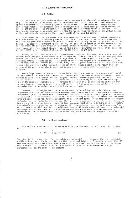
4.2 The Basic Equations
by:
At each step in the analysis, the vaniat.ion of plasma frequency FN with height H is given
NT
H - H A = : q 1 ( F N
J-r
FA )i \2)
The point FA,HA is the origin for the real-height polynornial. It is assumed that the real-height
profile is known up to the height HA; and that the vjrtual heights at frequencies greater than FA
have been cornected for the group delay of the rays in the underly'ing sections, to give the reduced
virtual heights h". The value of NT (the number of terms in the polynomial real-height
exoression) defines the order of the analysis.
L3