UAG-93: Chapters 1 to 5 - URSI

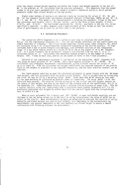
after the single virtual-height equation and before the single real-height equation in the set (7).
GA is the gradient at FA calculated from the previous polynomial. This departure from the normal
scheme is to g'ive exact agreement with the standarcj parabolic-lamjnation analysis, which matches
gradients rather than virtual heights at the end points.
Higher order methods of analysis are obtajned simply by increasing the values of NT, NV and
NR. For the standard fourth-order overlapp'ing polynomial analysis (Titheridge, 1967b) we set NT = 4,
NV = 3 and NR = 1. This gives a five term polynoniial (including the constant), fitted to the last
two calculated real heights h(k) [= HA] and h(k+1), and to the three virtual heights h'(k+1),
h'(k+2), and h'(k+:). The real*height expression for h(k+S), ava'ilable in the set (7), is not
specifically required. It does, however, give a good estimate of this height so that the correct
value of gyrofrequency can be used for the next step in the analysis.
4.3 Calculation Procedures
The subrout'ine C0EFIC (Appendix D.1) is called at each step to calculate the coefficients
B(i,j) for the simultaneous equations (.7). For the real-height conditions (5) the coefficients are
simple functions of frequency. The virtual-height equatjons involve group index integrals (4), which
are evaluated using 5- or 12-point Gaussjan integration depend'ing on the desired accuracy. At high
latitudes both 5 and 12 point'integrals are employed, over different sections of the integration
range, 'in a way which reduces errors by a factor of i0 to 100 at d'ip angles of 78 to 88' (Appendix
8.3). At a given frequency the NT polynomial integrals are obtained from the same 5, 12 or 17
calculated values of U'. Calculatjon time therefore depends primarily on the number of virtual
heights (NV) fitted at each step, and not on the number of terms in the fitted polynomial.
Solution of the simultaneous equations js carried out by the subroutine S0LVE (Appendix F.4).
This gives an exact solution if NT = NV+NR, and a least-square solution'if NT < NV+NR. The
calculation uses orthogonal Householder transformations, giving accurate results for values of NT
up to at least 15. From the calculated real-height coefficients any required features of the profile
(such as the heights or gradients at any required frequencies, and the total electron content) can be
obta i ned .
For least-squares solutions we want the calculated polynomial to agree closely with the NR known
real heights, and less accurately w.ith the given virtual heights. This is accomplished by multiplying
the first NV rows in (7) by a weighting factor WVIRT. Tests show that WVIRT should be less than
0.1 for good matching of successive polynomials under all conditions. The value WVIRT = 0.05 has
therefore been adopted. The relative fitting accuracies of the vjrtual and real heights depends on
the square of this weight, and also on the square of the relative size of the coeffic'ients B(i,j) in
the equations (7). Combining these effects gives a relative fitting accuracy of about 0.02. Thus for
a typical analysis us'ing real (inaccurate) data a calculated least-squares polynomial will fit the
previously determjned real heights to within about 0.01 km, and will agree with the virtual-height
data to w'ithin 0.5 km.
When an exact polynomial fit is bejng used (NT = NV+NR) or when real-height equations are not
included in the set being solved (as in the start or va11ey calculations) the value of WVIRT has no
effect on the results. When extraondinary ray data are bejng used to overcome the starting or va'l'ley
ambiguity additiona'l weights are used to give slightly less importance to the extraordinary ray
measurements, and greater importance to the last ordinary ray virtual height to ensure a smooth
continuation with fol lowinq ordinary rav measurements.
15