SOLUTIONS MANUAL for Stochastic Modeling: Analysis and ...

More documents

Recommendations

Info

100 CHAPTER 8. QUEUEING PROCESSES (e) Let the reneging rate be β =1/5 call/minute = 12 calls/hour for customers on hold. with µ = 20. µ i = { iµ, i =1, 2 2µ +(i − 2)β, i =3, 4,... (f) l q = ∑ ∞ j=3 (j − 2)π j Therefore, we need the π j for j ≥ 3. ⎧ ⎨ d j = ⎩ (λ/µ) j j! , j =0, 1, 2 2µ 2 ∏ j i=3 λ j (2µ+(i−2)β), j =3, 4,... 1 π 0 = ∑ ∞j=0 dj ≈ 1 ∑ 20 j=0 dj ≈ 1 2.77 ≈ 0.36 since ∑ n j=0 d j does not change in the second decimal place after n ≥ 20. Therefore 20 ∑ l q ≈ (j − 2)π j ≈ 0.137 calls on hold j=3 11. (a) M = {0, 1, 2,...,k+ m} is the number of users connected or in the wait queue. λ i = λ, i =0, 1,... { iµ, i =1, 2,...,k µ i = kµ +(i − k)γ, i = k +1,k+2,...,k+ m (b) l q = ∑ m j=k+1 (j − k)π j (c) λπ k+m (60 minutes/hour) (d) The quantities in (b) and (c) are certainly relevant. Also w q , the expected time spent in the hold queue. 12. We approximate the system as an M/M/3/20/20 with τ = 1 program/minute, and µ = 4 programs/minute λ i = µ i = { (20 − i)τ, i =0, 1,...,19 0, i =20, 21,... { iµ, i =1, 2 3µ, i =3, 4,...,20
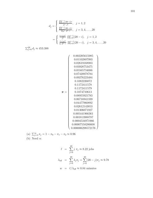
101 ∑ 20 j=0 d j ≈ 453.388 ⎧ ⎪⎨ d j = ⎪⎩ ⎧ ⎨ = ⎩ ∏ j−1 i=0 (20−i)τ , µ j j! ∏ j−1 j =1, 2 i=0 (20−i)τ , 3!µ j 3 3−j j =3, 4,...,20 (τ/µ) j j! ∏ j−1 i=0 (20 − i), j =1, 2 (τ/µ) j 63 3−j ∏ j−1 i=0(20 − i), j =3, 4,...,20 ⎛ π = ⎜ ⎝ (a) ∑ ∞ j=3 π j =1− π 0 − π 1 − π 2 ≈ 0.96 (b) Need w. 0.002205615985 0.01102807993 0.02619168983 0.03928753475 0.05565734086 0.07420978784 0.09276223484 0.1082226072 0.1172411578 0.1172411579 0.1074710613 0.08955921783 0.06716941339 0.04477960892 0.02612143853 0.01306071927 0.005441966361 0.001813988787 0.0004534971966 0.00007558286608 0.000006298572176 ⎞ ⎟ ⎠ l = λ eff = ∑20 j=0 ∑20 jπ j ≈ 8.22 jobs 20 ∑ λ j π j = (20 − j)π j ≈ 9.78 j=0 j=0 w = l/λ eff ≈ 0.84 minutes
Page 1 and 2:
SOLUTIONS MANUAL for Stochastic Mod
Page 3 and 4:
ii CONTENTS
Page 5 and 6:
Chapter 2 Sample Paths 1. The simul
Page 7 and 8:
3 7. Inputs: Number of hamburgers d
Page 9 and 10:
Chapter 3 Basics 1. (a) Pr{X =4} =
Page 11 and 12:
(b) 6. (a) F Y (a) = = ∫ a ⎧
Page 13 and 14:
9 (a) Pr{X 2 =1| X 1 =0} = Pr{X 2 =
Page 15 and 16:
11 16. Let U be a random variable h
Page 17 and 18:
13 Y = ⎧ ⎪⎨ ⎪⎩ 1, 0 ≤ U
Page 19 and 20:
15 (d) E[X] = ∑ all a ap X (a) =0
Page 21 and 22:
17 ( ) ∞∑ d 2 = γ a=1 dq 2 qa+
Page 23 and 24:
19 = ∫ ∞ −∞ ∫ ∞ a 2 f X
Page 25 and 26:
21 (b) Let T ≡ number of trials u
Page 27 and 28:
(b) f is maximized at a = β giving
Page 29 and 30:
Chapter 4 Simulation 1. An estimate
Page 31 and 32:
27 S n+1 ← S n − FD −1 endif
Page 33 and 34:
29 (b) Ȳ 1 = {0(5 − 0) + 1(6 −
Page 35 and 36:
Chapter 5 Arrival-Counting Processe
Page 37 and 38:
33 Pr{Y 2,6 > 30} = 1− Pr{Y 2,6
Page 39 and 40:
8. (a) Restricted to periods of the
Page 41 and 42:
37 Pr{Y (A) 1.5 > 1000,Y (B) 1.5 >
Page 43 and 44:
39 Pr{Y (B) 2 − Y (B) 1 > 5,Y (B)
Page 45 and 46:
41 (b) 20. (a) Pr{Y 52 − Y 48 =20
Page 47 and 48:
43 ⎧ ⎪⎨ λ(t) = ⎪⎩ 144, 0
Page 49 and 50:
while {b
Page 51 and 52:
27. We suppose that the time to bur
Page 53 and 54: and the latter with rate ( λ ′
Page 55 and 56: Chapter 6 Discrete-Time Processes 1
Page 57 and 58: 53 n =5 ⎛ ⎜ ⎝ 0.00001 0.68645
Page 59 and 60: 55 with ŝe = √ ̂p(1 − ̂p) 45
Page 61 and 62: 57 14. Case 6.3 S n represents the
Page 63 and 64: 59 Pr{≤ 1 defective} = a + b + c
Page 65 and 66: 61 ⎛ P = ⎜ ⎝ 0.92 0.08 0 0 0
Page 67 and 68: 63 25. (a) We first argue that µ 1
Page 69 and 70: 65 The expected number of spins is
Page 71 and 72: 67 = 1− Pr{X 1 >n} Pr{X 2 >n} = 1
Page 73 and 74: 69 = ∑ h∈A Pr{S 1 = j | S 0 = h
Page 75 and 76: 71 Therefore, the long-run expected
Page 77 and 78: 73 31. We show (6.5) for k = 2. The
Page 79 and 80: Chapter 7 Continuous-Time Processes
Page 81 and 82: 77 dp i3 (t) dt dp i4 (t) dt dp i5
Page 83 and 84: 79 endif C 2 ← T n+1 + FH −1 (r
Page 85 and 86: 81 8. See Exercise 7 for an analysi
Page 87 and 88: y conditioning on the first state v
Page 89 and 90: 85 0 0 0 0 0 0 0 0 0 0 0 0 0 0 0 0
Page 91 and 92: 87 or λµ 00 = 1 +λµ 10 λµ 01
Page 93 and 94: 89 e 2 () (order arrives from manuf
Page 95 and 96: 91 − λ M ∫ ∞ λ 1 + λ M t =
Page 97 and 98: Chapter 8 Queueing Processes 1. Let
Page 99 and 100: 95 λ i = µ i = { 20(1 − i/16),
Page 101 and 102: 97 (c) l q = ∞∑ π 2 + (j − 2
Page 103: We have assumed a 24-hour day, but
Page 107 and 108: 103 (c) For the M/M/s/c with s ≤
Page 109 and 110: will be at the front of the queue o
Page 111 and 112: 107 (b) For the M/M/1 For the M/D/1
Page 113 and 114: 109 = (1− ρ 1 )(1 − ρ 2 ) ∞
Page 115 and 116: 111 i a 0i µ (i) 1 20 30 2 0 30 (
Page 117 and 118: 113 or or ⎛ Λ[(I − R) ′ ]
Page 119 and 120: 115 i s i ρ i 1 19 0.88 2 4 0.75 3
Page 121 and 122: It appears that there will be very
Page 123 and 124: Chapter 9 Topics in Simulation of S
Page 125 and 126: 9. To obtain a rough-cut model, fir
Page 127 and 128: 123 w q =0.49hours l q = 3.2 trucks
Page 129 and 130: 125 When we fix the initial state,
show all

SOLUTIONS MANUAL for Stochastic Modeling: Analysis and ...

Create successful ePaper yourself

Delete template?

Save as template?