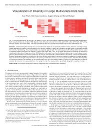
Integrated Computation of Finite Time Lyapunov Exponent During ...
Integrated Computation of Finite Time Lyapunov Exponent During ...
Integrated Computation of Finite Time Lyapunov Exponent During ...

You also want an ePaper? Increase the reach of your titles
YUMPU automatically turns print PDFs into web optimized ePapers that Google loves.
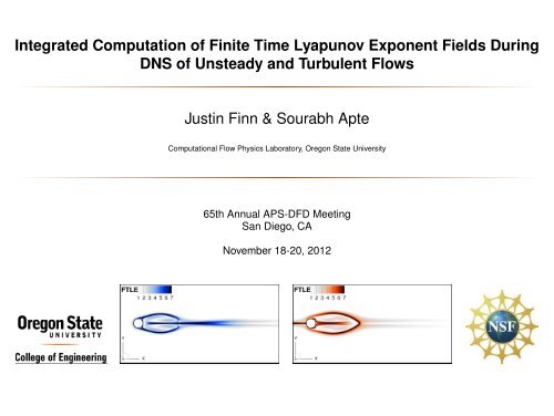
<strong>Integrated</strong> <strong>Computation</strong> <strong>of</strong> <strong>Finite</strong> <strong>Time</strong> <strong>Lyapunov</strong> <strong>Exponent</strong> Fields <strong>During</strong><br />
DNS <strong>of</strong> Unsteady and Turbulent Flows<br />
Justin Finn & Sourabh Apte<br />
<strong>Computation</strong>al Flow Physics Laboratory, Oregon State University<br />
65th Annual APS-DFD Meeting<br />
San Diego, CA<br />
November 18-20, 2012
Introduction<br />
<strong>Finite</strong> <strong>Time</strong> <strong>Lyapunov</strong> <strong>Exponent</strong> (FTLE)<br />
Avg. stretching rate <strong>of</strong> initially adjacent tracers over finite time.<br />
Ridges show strong correspondence with Lagrangian coherent<br />
structures (LCS): Invariant transport barriers, skeleton <strong>of</strong> tracer<br />
patterns. [Haller, 2001, Shadden et al., 2005]<br />
Relatively modern FTLE/LCS theory contributed new understanding to<br />
many fields<br />
Typically computed via algorithmically simple, computationally<br />
expensive post-processing <strong>of</strong> experimental/numerical data<br />
Enormous number <strong>of</strong> particle advections<br />
Careful memory management.<br />
Fewer velocity fields ⇒ more uncertainty.<br />
Speedup possible: AMR [Miron et al., 2012], Ridge<br />
tracking [Lipinski and Mohseni, 2010], GPU<br />
acceleration [Conti et al., 2012],<br />
Repelling<br />
trajectories [Shadden et al., 2005]<br />
Atmospheric events [Lekien and Ross, 2010] Granular flow in a tumbler [Christov et al., 2011]<br />
Startup <strong>of</strong> a swimming<br />
fish [Conti et al., 2012]<br />
Finn & Apte FTLE & DNS Integration 2
Main Goal: Enhance DNS capability<br />
Typical direct numerical simulation code<br />
̌□ Simulation resolves all space/time scales <strong>of</strong> the flow<br />
̌□ Massive parallelism, and rapidly growing processing power: New applications,<br />
larger simulations, complex configurations are possible.<br />
̌□ Particle/scalar tracking, interpolations, gradient calcs, etc...<br />
̌□ Low cost, high quality, on-the-fly FTLE computations<br />
Finn & Apte FTLE & DNS Integration 3
Main Goal: Enhance DNS capability<br />
Typical direct numerical simulation code<br />
̌□ Simulation resolves all space/time scales <strong>of</strong> the flow<br />
̌□ Massive parallelism, and rapidly growing processing power: New applications,<br />
larger simulations, complex configurations are possible.<br />
̌□ Particle/scalar tracking, interpolations, gradient calcs, etc...<br />
̌□ Low cost, high quality, on-the-fly FTLE computations<br />
One <strong>of</strong> our interests: How do porescale flow<br />
features affect mixing and transport in packed<br />
bed reactors<br />
Finn & Apte FTLE & DNS Integration 3
Main Goal: Enhance DNS capability<br />
Typical direct numerical simulation code<br />
̌□ Simulation resolves all space/time scales <strong>of</strong> the flow<br />
̌□ Massive parallelism, and rapidly growing processing power: New applications,<br />
larger simulations, complex configurations are possible.<br />
̌□ Particle/scalar tracking, interpolations, gradient calcs, etc...<br />
̌□ Low cost, high quality, on-the-fly FTLE computations<br />
Outline<br />
1 Definitions<br />
2 Our <strong>Integrated</strong> Approach<br />
3 2D & 3D examples<br />
4 Cost analysis<br />
One <strong>of</strong> our interests: How do porescale flow<br />
features affect mixing and transport in packed<br />
bed reactors<br />
Finn & Apte FTLE & DNS Integration 3
Definition and typical computation <strong>of</strong> the FTLE<br />
1 Release a grid <strong>of</strong> tracers and see where they go: This gives us the The flow map,<br />
Φ(x 0 , t 0 , )<br />
∫ t1<br />
Φ t 1<br />
t0<br />
(x 0 , t 0 ) = x 0 + u(x(τ), τ)dτ (1)<br />
t 0<br />
Finn & Apte FTLE & DNS Integration 4
Definition and typical computation <strong>of</strong> the FTLE<br />
1 Release a grid <strong>of</strong> tracers and see where they go: This gives us the The flow map,<br />
Φ(x 0 , t 0 , )<br />
∫ t1<br />
Φ t 1<br />
t0<br />
(x 0 , t 0 ) = x 0 + u(x(τ), τ)dτ (1)<br />
t 0<br />
2 Differentiate the flow map W.R.T. x 0 : Then, compose the right Cauchy-Green deformation<br />
tensor, ∆<br />
⎡<br />
⎤∗ ⎡ ⎤<br />
∆ t 1<br />
t0<br />
(x 0 , t 0 ) = ⎣ dΦt 1<br />
t0<br />
(x 0 , t 0 )<br />
⎦ ⎣ dΦt 1<br />
t0<br />
(x 0 , t 0 )<br />
⎦ , (2)<br />
dx 0<br />
dx 0<br />
3 Determine the largest eigenvalue <strong>of</strong> this tensor. This is then used to compute the<br />
(maximum) FTLE field.<br />
√<br />
σ t 1<br />
1<br />
t0<br />
(x 0 , t 0 ) =<br />
|t 1 − t 0 | log λ max (∆ t 1<br />
t0<br />
(x 0 , t 0 )) (3)<br />
4 Detect FTLE ridges visually or analytically: Forward time ridges ⇒ repelling LCS<br />
candidates. Backward time ridges ⇒ attracting LCS candidates. Recent, more exact<br />
theory [Haller, 2011]<br />
Note: Separate computations for forward (t 1 > t 0 ) and backward (t 1 < t 0 ) time<br />
Note: Let T be the absolute value <strong>of</strong> the integration time, |t 1 − t 0 |<br />
We can then write forward and backward time T flow maps as Φ t 0+T<br />
t and Φ t 0−T<br />
0<br />
t 0<br />
Finn & Apte FTLE & DNS Integration 4
The flow solver<br />
Originally developed for DNS/LES on very large grids in complex<br />
configurations [Moin and Apte, 2006],<br />
Distributed Memory (MPI) parallelization and good scalability to more than 1000<br />
processors.<br />
Co-Located (u, p known at cell centers), finite volume discretization<br />
Arbitrary cell shapes possible: Hex, tet, pyramid, etc...<br />
Fractional time-stepping, and Algebraic Multigrid (AMG) solver for pressure<br />
Poisson equation [Falgout and Yang, 2002]<br />
Extensions for Multiphase flow problems: Subgrid scale Euler-Lagrange<br />
models [Shams et al., 2010], Resolved rigid body motion with fictitious domain<br />
approach [Apte et al., 2009]<br />
Finn & Apte FTLE & DNS Integration 5
Computing the forward time flow map, Φ t 0+T<br />
t 0<br />
(3) Communicate<br />
Φ t0+T = x(t = t<br />
t0 0 + T )<br />
to take<strong>of</strong>f cell<br />
(2) Tracer advection<br />
to time t = t 0 + T<br />
The Lagrangian Treatment:<br />
1 Launch tracer from each<br />
cell center at t = t 0<br />
2 Update tracer position<br />
dx<br />
dt<br />
= u(x, t) (4)<br />
3 Communicate tracer<br />
position to launch cell<br />
(1) Launch tracers<br />
from cell centers,<br />
x(t = t 0 ) = x cv<br />
Finn & Apte FTLE & DNS Integration 6
Computing the forward time flow map, Φ t 0+T<br />
t 0<br />
(3) Communicate<br />
Φ t0+T = x(t = t<br />
t0 0 + T )<br />
to take<strong>of</strong>f cell<br />
(2) Tracer advection<br />
to time t = t 0 + T<br />
The Lagrangian Treatment:<br />
1 Launch tracer from each<br />
cell center at t = t 0<br />
2 Update tracer position<br />
dx<br />
dt<br />
= u(x, t) (4)<br />
3 Communicate tracer<br />
position to launch cell<br />
(1) Launch tracers<br />
from cell centers,<br />
x(t = t 0 ) = x cv<br />
Nothing new here, but what do we do about backward time<br />
Finn & Apte FTLE & DNS Integration 6
Computing the backward time flow map, Φ t 0<br />
t0 +T<br />
The Eulerian Treatment [Leung, 2011]: A natural way to evolve the backward time<br />
flow map in forward time. Treat each component <strong>of</strong> backward time flow map as an<br />
Eulerian scalar field on the fixed grid.<br />
dΦ t 0<br />
t0 +T ,i<br />
+ (u · ∇)Φ t 0<br />
t0 +T ,i<br />
= 0 (5)<br />
dt<br />
Solve three level-set equations using a simple, semi-Lagrangian<br />
scheme [Staniforth and Côté, 1991]<br />
At time t = t 0 , set<br />
Φ t0<br />
t0+T = x cv everywhere<br />
Evolve each<br />
scalar up to<br />
t = t 0 + T by<br />
solving level set<br />
equation.<br />
At time t = t 0 + T , Φ t0<br />
t0+T<br />
is the backward time T<br />
flow map.<br />
Finn & Apte FTLE & DNS Integration 7
Efficient composition <strong>of</strong> evolving FTLE fields<br />
When computing evolving FTLE fields, redundant tracer integrations eliminated by splitting time T<br />
flow map into N time h substeps.<br />
Φ t 0+T<br />
t 0<br />
Φ t 0+T<br />
t 0<br />
= Φ Nh<br />
(N−1)h ◦ · · · ◦ Φt 0+2h<br />
t 0 +h ◦ Φt 0+h<br />
t 0<br />
(6)<br />
= IΦ t 0+Nh<br />
t 0 +(N−1)h ◦ · · · ◦ IΦt 0+2h<br />
t 0 +h ◦ Φt 0+h<br />
t 0<br />
(7)<br />
[Brunton and Rowley, 2010]<br />
Finn & Apte FTLE & DNS Integration 8
Efficient composition <strong>of</strong> evolving FTLE fields<br />
Evolve time h flow maps during the simulation, store them on hard disk, construct time T flow<br />
maps as needed<br />
Approximate reconstruction <strong>of</strong> Φ t 0+2h+T<br />
t 0 +2h<br />
Approximate reconstruction <strong>of</strong> Φ t 0+h+T<br />
t 0 +h<br />
Approximate reconstruction <strong>of</strong> Φ t 0+T<br />
t 0<br />
}Fwd. time<br />
constructions<br />
Exact Φ t 0+T<br />
t 0<br />
t 0 t 0 +h t 0 +2h . . . . . . t 0 +T-h t 0 +T t 0 +h+T t 0 +2h+T<br />
Simulation<br />
<strong>Time</strong> (t)<br />
Exact Φ t 0<br />
t0 +T<br />
Approximate reconstruction <strong>of</strong> Φ t 0<br />
t0 +T<br />
Approximate reconstruction <strong>of</strong> Φ t 0+h<br />
t 0 +h+T<br />
}Bkwd. time<br />
constructions<br />
Approximate reconstruction <strong>of</strong> Φ t 0+2h<br />
t 0 +2h+T<br />
Finn & Apte FTLE & DNS Integration 8
<strong>Computation</strong>al flow <strong>of</strong> the integrated computations<br />
Main Flow Solver<br />
• t n+1 = t n + dt<br />
• Advance u n to u n+1<br />
Update time h flow maps<br />
• Advance time h<br />
Lagrangian tracers (fwd)<br />
• Advance time h Eulerian<br />
fields (bkwd)<br />
u n+1/2 mod (t n+1 , h) ≠ 0<br />
• Handle flow map B.C.<br />
RETURN<br />
mod (t n+1 , h) = 0<br />
FTLE <strong>Computation</strong><br />
• Map current tracer positions to<br />
launch cells to obtain time h<br />
forward flow map<br />
• Write time h flow maps to disk<br />
• Construct time T flow maps<br />
from sequence <strong>of</strong> N time h flow<br />
maps<br />
• Compute FTLE fields<br />
• Re-initialize time h flow maps<br />
on fixed grid.<br />
Block diagram showing the flow <strong>of</strong> the FTLE/DNS integration.<br />
Finn & Apte FTLE & DNS Integration 9
Demonstration<br />
We have tested our implementation for a number <strong>of</strong> flows:<br />
1<br />
<strong>Time</strong> dependent double gyre flow<br />
2<br />
The Karman vortex street behind a fixed cylinder<br />
3<br />
The oscillating cylinder problem<br />
4<br />
The traveling vortex ring<br />
5<br />
Unsteady flow through a randomly packed bed<br />
Finn & Apte FTLE & DNS Integration 10
Moving Boundaries: Inline Oscillation <strong>of</strong> a circular cylinder<br />
Re = UmD<br />
ν<br />
= 100 (6)<br />
KC = Um<br />
fD = 2πA<br />
D = 5 (7)<br />
Integraton time = 1.5 periods<br />
Temporal FTLE resolution , h = T /30<br />
x c(t) = −A m sin(2πft) (8)<br />
U c(t) = −2πAf cos(2πft) (9)<br />
Fictitious domain<br />
representation [Apte et al., 2009]<br />
Backward FTLE<br />
Forward FTLE<br />
Finn & Apte FTLE & DNS Integration 11
Three dimensional flows: Traveling vortex ring<br />
Three dimensional ring generated by<br />
circular inflow pulse<br />
660 × 241 × 241 stretched Cartesian<br />
grids (37M cells)<br />
FTLE computed for T = 1.5s: Ring<br />
travels 10% <strong>of</strong> the domain<br />
Temporal FTLE resolution, h = 0.1s<br />
2D Cross section <strong>of</strong> 3D FTLE field<br />
shows LCS candidates<br />
Backward FTLE<br />
Forward FTLE<br />
Finn & Apte FTLE & DNS Integration 12
Complex configurations: Flow through a randomly packed bed<br />
Weakly turbulent: Pore Reynolds<br />
number, Re = UD<br />
ɛν = 600<br />
Cartesian grid fictitious domain<br />
approach with grid spacing D/80<br />
in porespace<br />
integration time <strong>of</strong> T = 3U/D<br />
using a flow map sub-step <strong>of</strong><br />
h = T /7<br />
3D FTLE field visualized on 2D<br />
slices<br />
More detail in gallery <strong>of</strong> fluid<br />
motion poster<br />
Backward FTLE<br />
Forward FTLE<br />
Finn & Apte FTLE & DNS Integration 13
<strong>Computation</strong>al expense<br />
Simulation <strong>Time</strong> to compute evolving FTLE fields with T = 2400dt and h = T /12<br />
Fixed Cylinder (36 proc.)<br />
26.5%<br />
Oscillating Cylinder (24 proc.)<br />
22.8%<br />
Vortex Ring (660 proc.)<br />
14.2%<br />
Packed Bed (1200 proc.)<br />
16.1%<br />
0% 5% 10% 15% 20% 25% 30%<br />
Percentage <strong>of</strong> total simulation time<br />
Disk space and RAM:<br />
Largest case (Packed bed) required roughly 25GB or hard disk to store<br />
intermediate flow maps<br />
Minimal additional simulation RAM: Typically 10% or less <strong>of</strong> total computation<br />
Finn & Apte FTLE & DNS Integration 14
Conclusions<br />
1 We can compute evolving forward and backward time FTLE fields during direct<br />
numerical simulation <strong>of</strong> unsteady and turbulent flow<br />
2 The integration allows for high resolution FTLE computations, using the native<br />
space and time resolution <strong>of</strong> the simulation<br />
3 We have tested the implementation for 2D and 3D flows with both fixed & moving<br />
boundaries as well as complex configurations<br />
4 The FTLE computations contribute to 26% or less <strong>of</strong> the total simulation time, and<br />
require only moderate amounts <strong>of</strong> RAM/disk space.<br />
Future Work<br />
1 Precise extraction <strong>of</strong> LCS from developing theory<br />
2 Extension to inertial particles<br />
3 Simulations <strong>of</strong> FTLE based control<br />
Finn & Apte FTLE & DNS Integration 15
[Apte et al., 2009] Apte, S., Martin, M., and Patankar, N. (2009).<br />
A numerical method for fully resolved simulation (frs) <strong>of</strong> rigid particle-flow<br />
interactions in complex flows.<br />
Journal <strong>of</strong> <strong>Computation</strong>al Physics, 228(8):2712–2738.<br />
[Brunton and Rowley, 2010] Brunton, S. and Rowley, C. (2010).<br />
Fast computation <strong>of</strong> finite-time lyapunov exponent fields for unsteady flows.<br />
Chaos: An Interdisciplinary Journal <strong>of</strong> Nonlinear Science, 20(1):017503.<br />
[Christov et al., 2011] Christov, I., Ottino, J., and Lueptow, R. (2011).<br />
From streamline jumping to strange eigenmodes: Bridging the lagrangian and<br />
eulerian pictures <strong>of</strong> the kinematics <strong>of</strong> mixing in granular flows.<br />
Physics <strong>of</strong> Fluids, 23:103302.<br />
[Conti et al., 2012] Conti, C., Rossinelli, D., and Koumoutsakos, P. (2012).<br />
Gpu and apu computations <strong>of</strong> finite time lyapunov exponent fields.<br />
Journal <strong>of</strong> <strong>Computation</strong>al Physics, 231(5):2229–2244.<br />
[Falgout and Yang, 2002] Falgout, R. and Yang, U. (2002).<br />
hypre: A library <strong>of</strong> high performance preconditioners.<br />
<strong>Computation</strong>al ScienceICCS 2002, pages 632–641.<br />
[Haller, 2001] Haller, G. (2001).<br />
Distinguished material surfaces and coherent structures in three-dimensional fluid<br />
flows.<br />
Finn & Apte FTLE & DNS Integration 15
Physica D: Nonlinear Phenomena, 149(4):248–277.<br />
[Haller, 2011] Haller, G. (2011).<br />
A variational theory <strong>of</strong> hyperbolic lagrangian coherent structures.<br />
Physica. D, 240(7):574–598.<br />
[Lekien and Ross, 2010] Lekien, F. and Ross, S. (2010).<br />
The computation <strong>of</strong> finite-time lyapunov exponents on unstructured meshes and for<br />
non-euclidean manifolds.<br />
Chaos, 20(1):017505–1.<br />
[Leung, 2011] Leung, S. (2011).<br />
An eulerian approach for computing the finite time lyapunov exponent.<br />
Journal <strong>of</strong> computational physics, 230(9):3500–3524.<br />
[Lipinski and Mohseni, 2010] Lipinski, D. and Mohseni, K. (2010).<br />
A ridge tracking algorithm and error estimate for efficient computation <strong>of</strong> lagrangian<br />
coherent structures.<br />
Chaos, 20(1):017504–1.<br />
[Miron et al., 2012] Miron, P., Vétel, J., Garon, A., Delfour, M., and Hassan, M. (2012).<br />
Anisotropic mesh adaptation on lagrangian coherent structures.<br />
Journal <strong>of</strong> <strong>Computation</strong>al Physics.<br />
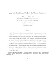
[Moin and Apte, 2006] Moin, P. and Apte, S. (2006).<br />
Large-Eddy Simulation <strong>of</strong> Realistic Gas Turbine-Combustors.<br />
Finn & Apte FTLE & DNS Integration 15
AIAA Journal, 44(4):698–708.<br />
[Shadden et al., 2005] Shadden, S., Lekien, F., and Marsden, J. (2005).<br />
Definition and properties <strong>of</strong> lagrangian coherent structures from finite-time lyapunov<br />
exponents in two-dimensional aperiodic flows.<br />
Physica D: Nonlinear Phenomena, 212(3-4):271–304.<br />
[Shams et al., 2010] Shams, E., Finn, J., and Apte, S. (2010).<br />
A numerical scheme for euler–lagrange simulation <strong>of</strong> bubbly flows in complex<br />
systems.<br />
International Journal for Numerical Methods in Fluids, 67:1865–1898.<br />
[Solomon and Gollub, 1988] Solomon, T. and Gollub, J. (1988).<br />
Chaotic particle transport in time-dependent rayleigh-benard convection.<br />
Physical Review A, 38(12):6280.<br />
[Staniforth and Côté, 1991] Staniforth, A. and Côté, J. (1991).<br />
Semi-lagrangian integration schemes for atmospheric models- a review.<br />
Monthly Weather Review, 119(9):2206–2223.<br />
Finn & Apte FTLE & DNS Integration 16
Double Gyre flow: [Solomon and Gollub, 1988]<br />
u = −πA sin(πf (x)) cos(πy) (10)<br />
v<br />
f<br />
a<br />
b<br />
= πA cos(πf (x)) sin(πy) ∂f<br />
∂x<br />
(x, t) = a(t)x 2 + b(t)x<br />
(t) = ɛ sin(ωt)<br />
(t) = 1 − 2ɛ sin(ωt)<br />
(11)<br />
ɛ = 0.1, A = 0.1, ω = 2π<br />
10<br />
512 × 256 Cartesian grid:<br />
0 ≤ X ≤ 2, 0 ≤ Y ≤ 1<br />
<strong>Time</strong> dependent 2d flow model in the X-Y plane<br />
Finn & Apte FTLE & DNS Integration 16
Double Gyre flow: [Solomon and Gollub, 1988]<br />
u = −πA sin(πf (x)) cos(πy) (10)<br />
v<br />
f<br />
a<br />
b<br />
= πA cos(πf (x)) sin(πy) ∂f<br />
∂x<br />
(x, t) = a(t)x 2 + b(t)x<br />
(t) = ɛ sin(ωt)<br />
(t) = 1 − 2ɛ sin(ωt)<br />
(11)<br />
Eulerian flow map captures sharp<br />
features.<br />
(a) t = 0 (b) t = 1.25<br />
ɛ = 0.1, A = 0.1, ω = 2π<br />
10<br />
512 × 256 Cartesian grid:<br />
0 ≤ X ≤ 2, 0 ≤ Y ≤ 1<br />
(c) t = 2.5 (d) t = 5<br />
(e) t = 10 (f) t = 15<br />
Finn & Apte FTLE & DNS Integration 16
Double Gyre flow: [Solomon and Gollub, 1988]<br />
u = −πA sin(πf (x)) cos(πy) (10)<br />
v<br />
f<br />
a<br />
b<br />
= πA cos(πf (x)) sin(πy) ∂f<br />
∂x<br />
(x, t) = a(t)x 2 + b(t)x<br />
(t) = ɛ sin(ωt)<br />
(t) = 1 − 2ɛ sin(ωt)<br />
ɛ = 0.1, A = 0.1, ω = 2π<br />
10<br />
512 × 256 Cartesian grid:<br />
0 ≤ X ≤ 2, 0 ≤ Y ≤ 1<br />
(11)<br />
Eulerian and Lagrangian results are<br />
equivalent<br />
(g) Backward time Lagrangian<br />
(h) Forward time Lagrangian<br />
(i) Backward time Eulerian (j) Forward time Eulerian<br />
(k) Backward time relative<br />
error<br />
(l) Forward time relative<br />
error<br />
Finn & Apte FTLE & DNS Integration 16
Flow past a fixed cylinder<br />
Backward FTLE<br />
Forward FTLE<br />
Finn & Apte FTLE & DNS Integration 17