Integrated Computation of Finite Time Lyapunov Exponent During ...
Integrated Computation of Finite Time Lyapunov Exponent During ...
Integrated Computation of Finite Time Lyapunov Exponent During ...

Create successful ePaper yourself
Turn your PDF publications into a flip-book with our unique Google optimized e-Paper software.
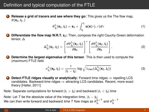
Definition and typical computation <strong>of</strong> the FTLE<br />
1 Release a grid <strong>of</strong> tracers and see where they go: This gives us the The flow map,<br />
Φ(x 0 , t 0 , )<br />
∫ t1<br />
Φ t 1<br />
t0<br />
(x 0 , t 0 ) = x 0 + u(x(τ), τ)dτ (1)<br />
t 0<br />
2 Differentiate the flow map W.R.T. x 0 : Then, compose the right Cauchy-Green deformation<br />
tensor, ∆<br />
⎡<br />
⎤∗ ⎡ ⎤<br />
∆ t 1<br />
t0<br />
(x 0 , t 0 ) = ⎣ dΦt 1<br />
t0<br />
(x 0 , t 0 )<br />
⎦ ⎣ dΦt 1<br />
t0<br />
(x 0 , t 0 )<br />
⎦ , (2)<br />
dx 0<br />
dx 0<br />
3 Determine the largest eigenvalue <strong>of</strong> this tensor. This is then used to compute the<br />
(maximum) FTLE field.<br />
√<br />
σ t 1<br />
1<br />
t0<br />
(x 0 , t 0 ) =<br />
|t 1 − t 0 | log λ max (∆ t 1<br />
t0<br />
(x 0 , t 0 )) (3)<br />
4 Detect FTLE ridges visually or analytically: Forward time ridges ⇒ repelling LCS<br />
candidates. Backward time ridges ⇒ attracting LCS candidates. Recent, more exact<br />
theory [Haller, 2011]<br />
Note: Separate computations for forward (t 1 > t 0 ) and backward (t 1 < t 0 ) time<br />
Note: Let T be the absolute value <strong>of</strong> the integration time, |t 1 − t 0 |<br />
We can then write forward and backward time T flow maps as Φ t 0+T<br />
t and Φ t 0−T<br />
0<br />
t 0<br />
Finn & Apte FTLE & DNS Integration 4