A Firmware-Based Polyphase Filter Design Tool - University of Cape ...

A Firmware-Based Polyphase Filter Design Tool
Prepared by:
David George
Fourth Year Electrical and Computer Engineering Student
University of Cape Town
17th October 2005

Declaration
I declare that this project report is my own, unaided work. It is a project report submitted
to the Department of Electrical Engineering, The University of Cape Town, in partial
fulfilment of the requirements for the degree of Bachelor of Science in Engineering. It
has not been submitted before for any degree or examination at any other university.
Signature of Author . . . . . . . . . . . . . . . . . . . . . . . . . . . . . . . . . . . . . . . . . . . . . . . . . . . . . . . . . . . . . .
Cape Town, 17th October 2005
i

Abstract
Polyphase filters are highly efficient structures for channelizing signals. When applied
in firmware they are capable of running at very high data rates, owing to the parallelism
they allow. This project’s primary aim was to develop a firmware-based polyphase filter
design tool, using open source tools wherever possible. The project went through three
stages of development: first, mathematical simulations were coded, second, a firmware
design was developed and finally, the design was implemented on a USRP GNU Radio
board. A simulation environment was developed to create a uniform way of applying
and retrieving signals throughout these stages, which aided the testing and analysis of the
polyphase filter’s design. Potential improvements and optimizations are discussed in the
conclusions.
ii

Acknowledgements
I would like to thank Alan Langman for his help and guidance throughout the project.
Thanks also to Marc Welz and Andrew Martens for all the help they gave. I also wish to
thank my mother for unscrambling my “eccentric use of the English language”.
Finally, I would like to thank my supervisor, Professor Mike Inggs, for his advice and
constant encouragement.
iii

Contents
Declaration
Abstract
Acknowledgements
Glossary
i
ii
iii
x
1 Introduction 1
1.1 Project Background . . . . . . . . . . . . . . . . . . . . . . . . . . . . . 1
1.2 Objectives of the Project . . . . . . . . . . . . . . . . . . . . . . . . . . 1
1.2.1 Coding Mathematical Simulations . . . . . . . . . . . . . . . . . 1
1.2.2 Creating a Simulation Environment . . . . . . . . . . . . . . . . 2
1.2.3 Designing PFBs in Verilog . . . . . . . . . . . . . . . . . . . . . 2
1.2.4 Implementing the Design on and FPGA . . . . . . . . . . . . . . 2
1.3 Scope and Limitations . . . . . . . . . . . . . . . . . . . . . . . . . . . 3
1.4 Document Outline . . . . . . . . . . . . . . . . . . . . . . . . . . . . . . 4
2 Concepts Overview 5
2.1 Digital Filter Design . . . . . . . . . . . . . . . . . . . . . . . . . . . . 5
2.1.1 Finite Impulse Response[FIR] Filters . . . . . . . . . . . . . . . 5
2.1.2 Filter Characteristics . . . . . . . . . . . . . . . . . . . . . . . . 5
2.1.2.1 Magnitude Response . . . . . . . . . . . . . . . . . . 6
2.1.2.2 Phase Response . . . . . . . . . . . . . . . . . . . . . 6
2.1.3 The Windowing Method of FIR Filter Design . . . . . . . . . . . 7
2.2 Polyphase Filter Theory . . . . . . . . . . . . . . . . . . . . . . . . . . . 8
2.2.1 Conventional Digital Channelizer . . . . . . . . . . . . . . . . . 8
2.2.2 Polyphase Filters . . . . . . . . . . . . . . . . . . . . . . . . . . 10
iv

3 Simulation Environment and Mathematical Simulations 12
3.1 The Simulation Environment . . . . . . . . . . . . . . . . . . . . . . . . 12
3.1.1 Motivation . . . . . . . . . . . . . . . . . . . . . . . . . . . . . 12
3.1.2 Design . . . . . . . . . . . . . . . . . . . . . . . . . . . . . . . 12
3.2 Mathematical Simulations . . . . . . . . . . . . . . . . . . . . . . . . . 14
3.2.1 Simulation Parameters . . . . . . . . . . . . . . . . . . . . . . . 14
3.2.2 Frequency Sweep Response . . . . . . . . . . . . . . . . . . . . 15
3.2.3 Frequency Comb Response . . . . . . . . . . . . . . . . . . . . . 15
4 Firmware Design 17
4.1 Firmware Modules . . . . . . . . . . . . . . . . . . . . . . . . . . . . . 17
4.1.1 FIR Filter . . . . . . . . . . . . . . . . . . . . . . . . . . . . . . 17
4.1.1.1 Basic Hardware . . . . . . . . . . . . . . . . . . . . . 17
4.1.1.2 Pipelined Hardware . . . . . . . . . . . . . . . . . . . 18
4.1.2 FFT . . . . . . . . . . . . . . . . . . . . . . . . . . . . . . . . . 18
4.1.2.1 Combinational Hardware . . . . . . . . . . . . . . . . 19
4.1.2.2 Pipelined Hardware . . . . . . . . . . . . . . . . . . . 19
4.1.3 JFFT . . . . . . . . . . . . . . . . . . . . . . . . . . . . . . . . 20
4.2 Overall System Design . . . . . . . . . . . . . . . . . . . . . . . . . . . 20
4.2.1 Combinational Design . . . . . . . . . . . . . . . . . . . . . . . 21
4.2.2 Pipelined Design . . . . . . . . . . . . . . . . . . . . . . . . . . 21
4.2.3 Mixed Design . . . . . . . . . . . . . . . . . . . . . . . . . . . . 22
4.3 Design Parameters . . . . . . . . . . . . . . . . . . . . . . . . . . . . . 22
4.3.1 Number of Channels . . . . . . . . . . . . . . . . . . . . . . . . 23
4.3.2 Prototype Filter . . . . . . . . . . . . . . . . . . . . . . . . . . . 23
4.3.3 Input Word length . . . . . . . . . . . . . . . . . . . . . . . . . 23
4.3.4 Output Word length . . . . . . . . . . . . . . . . . . . . . . . . . 24
4.4 Testing and Validation . . . . . . . . . . . . . . . . . . . . . . . . . . . 24
4.4.1 Frequency Sweep Response . . . . . . . . . . . . . . . . . . . . 24
4.4.2 Frequency Comb Response . . . . . . . . . . . . . . . . . . . . . 24
4.4.3 Effect of Input Word Length . . . . . . . . . . . . . . . . . . . . 25
v

5 Firmware Implementation 28
5.1 The USRP System . . . . . . . . . . . . . . . . . . . . . . . . . . . . . 28
5.1.1 USRP Hardware . . . . . . . . . . . . . . . . . . . . . . . . . . 28
5.1.1.1 AD and DA Converters . . . . . . . . . . . . . . . . . 28
5.1.1.2 Daughter Boards . . . . . . . . . . . . . . . . . . . . . 30
5.1.1.3 USB Controller . . . . . . . . . . . . . . . . . . . . . 30
5.1.2 USRP Firmware . . . . . . . . . . . . . . . . . . . . . . . . . . 30
5.1.3 USRP Software . . . . . . . . . . . . . . . . . . . . . . . . . . . 32
5.2 Polyphase Filter Implementations . . . . . . . . . . . . . . . . . . . . . 33
5.2.1 ROM Signal File . . . . . . . . . . . . . . . . . . . . . . . . . . 33
5.2.1.1 Results . . . . . . . . . . . . . . . . . . . . . . . . . . 33
5.2.2 An FM Radio Channel Browser . . . . . . . . . . . . . . . . . . 34
5.2.2.1 Results . . . . . . . . . . . . . . . . . . . . . . . . . . 35
6 Conclusions and Recommendations 38
Appendix A 39
Appendix B: Source Code 41
Bibliography 42
vi

List of Figures
1.1 The USRP Board . . . . . . . . . . . . . . . . . . . . . . . . . . . . . . 3
2.1 Filter Design Specifications . . . . . . . . . . . . . . . . . . . . . . . . . 6
2.2 Sinc Function Truncated in Time . . . . . . . . . . . . . . . . . . . . . . 7
2.3 Performance of Three Window Functions . . . . . . . . . . . . . . . . . 8
2.4 The Conventional Digital Channeliser . . . . . . . . . . . . . . . . . . . 9
2.5 The Channelising Process . . . . . . . . . . . . . . . . . . . . . . . . . . 9
2.6 The DFT Filter Bank . . . . . . . . . . . . . . . . . . . . . . . . . . . . 11
2.7 Input Commutator Model of a Polyphase Filter Bank . . . . . . . . . . . 11
3.1 The Simulation Environment’s Conceptual Design . . . . . . . . . . . . . 13
3.2 Rectified Frequency Sweep Response of Mathematical Simulation . . . . 15
3.3 Frequency Comb Magnitude and Phase Response . . . . . . . . . . . . . 16
4.1 Architecture of a FIR Filter . . . . . . . . . . . . . . . . . . . . . . . . . 17
4.2 [a] Rearranged Adders [b] Pipelined FIR Filter . . . . . . . . . . . . . . 18
4.3 Signal Flow Graph for a 4-Point FFT . . . . . . . . . . . . . . . . . . . . 19
4.4 R2MDC Architecture with N equals 8 . . . . . . . . . . . . . . . . . . . 20
4.5 Polyphase Filter with Combinational FIR Filter Bank and FFT . . . . . . 21
4.6 Polyphase Filter with both FIR Filter Bank and FFT Pipelined . . . . . . 22
4.7 The Implemented Polyphase Filter Design . . . . . . . . . . . . . . . . . 23
4.8 Frequency Sweep Response of Verilog Polyphase Filter . . . . . . . . . . 24
4.9 Frequency Comb Response of Verilog Polyphase Filter . . . . . . . . . . 25
4.10 Frequency Comb Response with Various Input Word Lengths . . . . . . . 26
4.11 Frequency Sweep Response with a Word Length of 8 . . . . . . . . . . . 27
5.1 USRP Hardware Block Diagram . . . . . . . . . . . . . . . . . . . . . . 29
vii

5.2 The USRP Firmware . . . . . . . . . . . . . . . . . . . . . . . . . . . . 31
5.3 The USRP Firmware Receive Path . . . . . . . . . . . . . . . . . . . . . 32
5.4 Implementation of a the Polyphase Filter Using a Signal ROM . . . . . . 33
5.5 Firmware Implementation Results with Signal Stored in a ROM File . . . 34
5.6 Firmware for a Radio Channel Browser . . . . . . . . . . . . . . . . . . 35
5.7 The GNU Radio FM Radio Receiver with Polyphase Filter Channels Overlayed
. . . . . . . . . . . . . . . . . . . . . . . . . . . . . . . . . . . . . 36
5.8 The First Eight Outputs of the Channel Browser . . . . . . . . . . . . . . 37
viii

List of Tables
3.1 Simulation Units Used in this Project . . . . . . . . . . . . . . . . . . . . 14
ix

Glossary
Decimation — A digital signal processing operation that reduces data rates by only retaining
every Mth sample, where M is the decimation factor.
Mixing — A signal processing operation that shifts a signal in the frequency domain by
multiplicating it in time with a local oscilator.
FPGA — A programmable logic device that uses programmable gate array technology to
process digital information.
Firmware — Software that is embedded in a hardware device. Firmware has been used as
the term to describe the code used to programme an FPGA.
Software-defined Radio — A radio system that uses software to perform the modulation
and demodulation of signals.
Open Source — A philosophy that promotes the access and improvement of a product’s
source.
x

Chapter 1
Introduction
1.1 Project Background
Digital signal processing [DSP] is an electrical engineering field whose existence is rapidly
becoming ubiquitous in our modern lives. It is applied in the fields of medicine, computing
and entertainment, to name a few. Given DSP’s practical use and the fact that
developments in DSP research and techniques are frequent, it stands out as a subject to
study. The DSP field that this project focuses on is multirate signal processing. More
specifically, the project will involve polyphase filter bank theory.
Polyphase filter banks [PFBs], or polyphase filters, are frequently used in high speed data
processing. They provide an extremely efficient means of separating signals into multiple
channels, as will be seen later. Polyphase filters have many applications, two examples
of which are in lossy audio compression techniques, such as the well known MP3 format,
and in digital spectrum analysers.
1.2 Objectives of the Project
Currently, there are many proprietary tools that can simulate, generate and test polyphase
filters. However, these tools can be prohibitively expensive for amateur radio enthusiasts,
academic institutions and small businesses. The high-level objective of this project was
to develop a tool to generate and test firmware-based polyphase filter banks, using open
source software wherever possible.
To achieve this objective, the project was broken down into the following tasks:
1.2.1 Coding Mathematical Simulations
The first step in approaching the problem was to write a polyphase filter bank simulation
derived from polyphase filter theory. The first purpose of this task was to provide insight
1

into how PFBs work. The second purpose of these simulations was to provide a reference
for later results obtained from Hardware Description Language [HDL] and Field
Programmable Gate Array [FPGA] simulations. With this reference, the correctness of
the latter designs was gauged.
A subtask of the mathematical simulations was to write a Finite Impulse Response [FIR]
filter prototype generator. The FIR filter prototype governs how well the polyphase filter
works. Thus, this subtask played an important role in the implementation of the project
as a complete polyphase filter bank creation tool.
1.2.2 Creating a Simulation Environment
Being able to test a design and to show correctness is essential to any design project. To
make testing easier, a simulation environment was developed to link to the various simulations
and hardware implementations. The simulation environment provided a uniform
way of loading parameters and applying and retrieving signals to and from these simulations.
The shell of the environment was coded in Python, with the internals coded in C
for performance.
1.2.3 Designing PFBs in Verilog
The first part of this task was to consider designs of the FIR filter and Fast Fourier Transform
[FFT] modules for a polyphase filter. After this, a top level design was developed,
which linked these modules. The Verilog HDL code that describes the PFB design was
made to be generated automatically from a set of parameters.
In order to test the designs, the Verilog simulator was linked to the simulation environment.
This allowed for tests of correctness, as well as for the analysis of the performance
of the design.
1.2.4 Implementing the Design on and FPGA
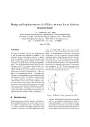
The Verilog PFB code was used to alter the firmware of a GNU Radio Universal Software
Radio Peripheral [USRP] Revision 3 board, shown in Figure 1.1. This board includes an
Altera Cyclone FPGA, high speed Analogue-to-Digital Converters [ADCs] and Digitalto-Analogue
Converters [DACs] and a Universal Serial Bus [USB] 2.0 interface. Quartus
Web Edition was be used to programme the FPGA and was the only proprietary tool used
throughout the project. The USRP system includes C++ code, which interfaces with the
board.
Two tests were performed to analyse the implementation. The first test involved sending
a digital input signal to the firmware based-polyphase and transmitting the filter’s output
2

ack to the host Personal Computer [PC], both via the USB link. Both input and output
signals were handled by the simulation environment. The second test involved utilizing
the PFB design to create a Frequency Modulation [FM] radio signal channel browser.
Figure 1.1: The USRP Board
1.3 Scope and Limitations
There was little emphasis throughout this project on creating an optimal design. Instead,
the aim was to generate a correct generic design.
This project entailed the application of a wide range of skills relating to software, firmware
and hardware. Many of these skills had to be learned through the course of the project, a
process that was time-consuming, as was the hardware interfacing and the application of
the GNU Radio Python code. For this reason, many project details and potential solutions
could not be investigated in depth in this research.
3

1.4 Document Outline
Chapter 2 provides a brief overview of concepts involved in the project. First, it describes
basic digital filters and the filter characteristics that are design considerations. Second,
it presents the FIR filter design methods used in this research. The chapter also briefly
describes polyphase filter theory. It presents a polyphase filter as being a highly efficient
channelizer.
Chapter 3 details the simulation environment design and presents results from the mathematical
simulations. It discusses the benefits of developing a simulation environment,
with the primary benefit being that of improved testability. The mathematical simulation
results are presented as an example of how the simulation environment is used. These
results also provide the correct reference for later simulations.
Chapter 4 details the Verilog design and simulations. The design is first analysed on a
component level, with potential designs for primary elements reviewed. The next step
is a review of three top-level designs, a combinational, a pipelined and a mixed design.
The mixed design is chosen for its efficiency and simplicity. The same tests that were
run on the mathematical simulation were run on Verilog simulations. There is also an
investigation into word length design parameters.
Chapter 5 gives details of the design implemented on the USRP board. It first provides
a brief background of the USRP system and GNU Radio. Then it describes the standard
firmware of the USRP system. Two tests are set up to analyse the performance of the PFB
design. The first test sets up a Read Only Memory [ROM] structure, with values loaded
from the simulation environment, which are then passed through to the polyphase filter.
The output of the filter is sent for analysis to the simulation environment on the host PC
via the USB link. In the second test, the developed polyphase filter is used as an FM radio
channel browser. The Python GNU Radio software is used to analyse the outputs.
Chapter 6 contains conclusions and recommendations based on the results.
4

Chapter 2
Concepts Overview
2.1 Digital Filter Design
There is a continuing trend of using digital rather than analogue methods in modern signal
processing. This is because digital systems are often more effective than their analogue
counterparts in, for example, their simulatability and their total stability in the face of
temperature change and component drift. They are also versatile and can be more easily
customized[1].
2.1.1 Finite Impulse Response[FIR] Filters
A FIR filter is a a type of digital filter that is characterized by its filter coefficients, h[n].
h[n] is a finite length vector of real numbers. The output of a system, y[n], is calculated
by convolving the input of the system, x[n], with the filter coefficients. Thus, the output
of a system can be stated as follows[1]:
y[n] =
N−1
∑ h[k]x[n − k] (2.1)
k=0
FIR filters are desirable because they can exhibit exact linear phase. For this reason, FIR
filters are the only type of digital filter investigated in this project.
2.1.2 Filter Characteristics
Both digital and analogue filters have the characteristic of removing or filtering ranges of
input frequencies. The frequency response of a filter is a description of how a filter affects
input signals at various frequencies. The frequency response can be separated into three
bands: the pass-band, the stop-band and the transition-band. The pass-band is the range
of frequencies that the filter lets through. The stop-band is the range of frequencies that
5

the filter fully attenuates and the transition-band is the range of frequencies that is only
partially attenuated. Filters are named by their pass-band. For example, low-pass filters
let through the low frequencies and high-pass filters let through the high frequencies.
The frequency response of a filter is a combination of its magnitude response and its phase
response.
2.1.2.1 Magnitude Response
The magnitude response, |H(e jw )|, of a filter is the amount the filter scales different frequencies.
Ideally, the magnitude response would be equal to 1 in the pass-band and 0 in
the stop-band. However, this is impossible as it would require a filter of infinite length.
Thus, other design considerations need to be made. Figure 2.1 shows the design specifications
for the magnitude response of a filter[2].
Figure 2.1: Filter Design Specifications
The pass-band and stop-band magnitude responses and cut-off frequencies are primary
design considerations. The ripple presence on the pass-band and stop-band is also of
significance.
2.1.2.2 Phase Response
The phase response of a filter is an indication of the time delay experienced by input
frequencies. The derivative of the phase response gives the group delay, which is a measurement
of how much the frequency components are delayed.
If the phase response of a filter is non-linear, frequency components will be delayed differently.
This causes signals to be smeared in time, which can badly degrade them. However,
6

&('
$
!"
if the phase response is linear, the delay of all frequencies is equal. Thus, a delayed but
preserved signal is produced.
2.1.3 The Windowing Method of FIR Filter Design
The ideal low pass filter would have a magnitude response of 1 in the pass-band and
0 in the stop-band and would have a 0 width transition-band. In the time domain this
filter would be an infinitely long sinc function. This is obviously not possible as it would
require infinite multipliers and adders in order to implement. A solution to this is to
truncate the time domain function to a certain number of samples. Figure 2.2 shows the
results of this solution. This method shows very undesirable filter attributes, including a
very large pass-band ripple, which increases in magnitude towards the band edge, owing
to the Gibbs[3] phenomenon and a very large stop-band ripple.
)+*-,/.102341576-8:9+;31.@0 .=

\[
^Z]
VW
YZ X
_
[
Z
Š^Z
‹Œ X
\[
NKTUL
NKTUM
LRTUL
LRTUM
LRTU‰
NKTUL
LRT w
LRT v
LRTU‰
NKTUL
LRT w
LRT v
LRTUL
LRTUO
t ORL
t NKL
t¥w L
t QRL
t¥v L
t MRL
t¥v L
t¥w L
L
L
t NKLPL
t MRL
t ORLPL
t NKMPL
t MRL
L
t NKMPL
t NKLPL
t ORMPL
t ORLPL
L
L N O Q w M v†u
L N O Q w M v†u
€ˆ|~‚+ƒgf~ce‚+|
o¢|~{
jm{-|H}gle|~cen
jma‡
€B|H‚+ƒgfice‚+|
jm{-|H}gle|~cen
`xacedgfihyjzleceno¢afic
q=dg„…s
q=dg„…s
apfic
hrqces
`bacedgfihkjmlecenö
ORTUL
L
MRL
t Q t O t N L N O Q
t¥u L
L M NKL N¢M OPL OPM QRLSQRM
t ORMPL
MRL
t NKLPL
t MRL
LRTUL
LRTUO
t ORLPL
t NKMPL
L M NKL N¢M OPL OPM QRLSQRM
t Q t O t N L N O Q
t QRLPL
t ORL
t MRL
ŽZ Œ Œ
t NKOPL
t NKLPL
t ‰RL
L t NKLPL
Q w M v†u
O N L
t NKMPL
t N w L
t ORLPL
t Q t O t N L N O Q
L M NKL N¢M OPL OPM QRLSQRM
¥‘’:“/”R’ P•–r— ‘˜:/š
¥‘’:“/”R’ R•–›— ‘˜+/š
Figure 2.3: Performance of Three Window Functions
on both the pass-band and stop-band. The rectangular window has the narrowest main
lobe but it has a very poor side-lobe response. Hence, it generates a filter with a small
transition-band, but with poor attenuation in the stop-band and poor ripple response. The
Blackman window has a wide main lobe and very low side lobes. This leads to a large
transition-band, but also to substantial attenuation of the stop-band. The Hamming window
introduces a parameter that adjusts the height of a discontinuity on the edge of its
raised cosine shape, which allows the side-lobe levels to be selected.
2.2 Polyphase Filter Theory
2.2.1 Conventional Digital Channelizer
A channelizer is a system that takes in a single signal consisting of several frequency
division multiplexed channels and generates output signals corresponding to each channel
converted to baseband. Figure 2.4 shows the conventional channelizer architecture.
Each complex multiplier shifts that channel’s signal in the frequency domain by 2πk/M,
where M is the number of channels and k is the channel number. The low-pass filter
extracts a single channel, while the decimator compresses the spectrum into baseband.
The process is summarized in Figure 2.5. The performance of the channelizer relies
greatly on the design of the prototype low-pass filter.
8

Figure 2.4: The Conventional Digital Channeliser
Figure 2.5: The Channelising Process
9

It is important to note the computational complexity of this method. The conventional
channelizer must implement M parallel low-pass filters of order N − 1 at the frequency of
the input sample rate.
2.2.2 Polyphase Filters
The fundamental theory behind polyphase filters is the polyphase decomposition. This
states that a filter, H(z), can be represented in the M-component polyphase form[2]:
H(z) =
M−1
∑ z −k E k (z M ) (2.3)
k=0
E k (z) are called the polyphase components and their inverse Z-transforms, e k [n], are given
by the following equation[2]:
e k [n] = h[nM + k] (2.4)
Thus, the polyphase components can be described in terms of a prototype filter h[n].
By replacing h[n] with a generalized up-converted filter, h[n]e jΘ kn , the following equation
for a uniform DFT filter bank can be derived[2]:
H k (z) =
M−1
∑ W −kn z −n E n (Z m ) (2.5)
n=0
This equation describes the architecture shown in Figure 2.6, which contains a bank of
FIR filters with increasingly delayed inputs, the output of which serves as the inputs to
an Inverse Discrete Fourier Transform [IDFT]. It can be observed that if the number of
channels M is a power of 2 the IDFT can be replaced by an Inverse Fast Fourier Transform
[IFFT].
Figure 2.7 shows the Input Commutator Model of a polyphase filter. This model is derived
through the addition of a decimation operation into the system as described in [6].The
input commutator model formed the basis for the project designs.
10

Figure 2.6: The DFT Filter Bank
Figure 2.7: Input Commutator Model of a Polyphase Filter Bank
11

Chapter 3
Simulation Environment and
Mathematical Simulations
3.1 The Simulation Environment
3.1.1 Motivation
Completing this project required that the following designs be verified:
• Mathematical Polyphase Filter Simulation
• Polyphase Filter HDL Code
• Implementation of HDL code on FPGA
Each one of these project elements receive inputs and produce outputs in an identical
format. It was a logical decision to create an environment that could manage and automate
the handling signals.
Management of signals would be of great benefit. It would allow identical signals to be
applied to project elements and their outputs to be processed from a single environment.
This would make it very simple to analyse the performance of a design with respect to a
correct reference. An example of such a reference could be a mathematical simulation.
Thus, a simulation environment would make it easier to verify and analyse designs.
3.1.2 Design
The design of the simulation environment was fairly simple. Figure 3.1 shows the basic
concept of the system design.
12

Figure 3.1: The Simulation Environment’s Conceptual Design
13

The simulation environment has the following primary elements:
• Signals
• Sinks
• Parameters
• Simulation Units
Signals serve as inputs and the sinks serve as outputs to simulation units. Parameters are
a static valued structure passed to the simulation units. Simulation units contain the core
process to be run. The simulation units were coded in C for performance, while the other
elements were developed in Python for the convenience that scripting languages provide.
The simulation units developed in this project are summarized in Table 3.1. The names
of these units are used when running a process in the simulation environment.
Table 3.1: Simulation Units Used in this Project
Name
C_POLY_SIM
V_FFT_SIM
V_POLY_SETUP
V_POLY_SIM
F_POLY_SETUP
F_POLY_READ
Description
Mathematical polyphase filter simulation
Verilog simulation of 64 point FFT
Setup the Verilog polyphase filter simulation
Verilog polyphase filter simulator
Setup the signal ROM firmware implementation
Reads back the signals from the firmware Implementation
3.2 Mathematical Simulations
This section will present the results of a C-coded simulation, based on the mathematical
description of a polyphase filter bank. These results are critical as they form a reference
for later HDL and hardware implementations. The section dually serves as a results section
for the simulation environment, as the C simulation was coded as a simulation unit.
3.2.1 Simulation Parameters
The mathematical simulations require two parameters: number of channels and prototype
FIR filter. These are passed from the simulation environment to the simulation unit via the
parameters structure. The prototype FIR filter is generated by the filter generation tool.
14

³ž
³
œ³´
³œ
œ³
œ³¢
œ³œ
œ³ž
3.2.2 Frequency Sweep Response
To test the performance of a polyphase filter a logical test would be to sweep a sinusoidal
frequency across the entire input band. This test would show how each channel responded
only when the sweep were present in its band. The envelope of the response should be
equal to the magnitude response of the filter prototype.
Figure 3.2 shows the simulation results of a frequency sweep across the input of an eight
channel polyphase filter. These results clearly show the out-of-band attenuation expected.
In addition, the envelope forms the shape of the prototype filter, which in this case was a
64-point Blackman window.
¾=¿¥ÀªÁÂUÁ¿ÄÃÆÅ=Ç ¿¥È@ɨ¿¢Ê¨Ë¨ÌBÍÎR¿¥¿¢Ïо=¿¥ÑÒÏӨʨѪ¿
³¢
¼½
µ·¸
¹º»
ž Ÿ ¡ ¢
œ
¦¨§ª©¦¨«¬®­i¯ ¤ °¨±ª² £¥¤
Figure 3.2: Rectified Frequency Sweep Response of Mathematical Simulation
3.2.3 Frequency Comb Response
This test involved applying several equally spaced frequency components into the polyphase
filter simulation. The range of frequency values were chosen to span a single channel,
specifically where M = 0.
Figure 3.3 shows the magnitude and phase response of the output channel of interest,
where M = 0. The magnitude response of the frequency comb exhibits a very similar
response to that of the prototype filter. The magnitude response of the prototype filter is
shown in red.
The phase response shown in Figure 3.3 was obtained by sampling the real output phase
response at the comb frequencies. It shows clearly that the linear-phase of the prototype is
almost entirely retained. There are minor deviations from the ideal phase and magnitude
responses. Identical deviations were encountered by Harris, as shown in [6].
15

ðñ
ôóðò
éêë
íîïì
ê ð
ô
ò
©ê
ñ
Ô
ýBþ~ÿ¡ £¢ˆ÷¥¤§¦gþ~ú¨¤+÷
õmö-÷Høgùe÷~úeûü
ÖRÔ
ç ÖPÔ
Ô
ç ÚPÔ
ç ØPÔ
ç Õ¢ÔRÔ
ç¥è Ô
Õ Ö × Ø Ù Ú
Ô
Û@ÜÝ:Þ/ßPÝ:àRáâ›ã¥Üä:åRæ
ç Ù
ç Õ¢Ô
ç Õ¢Ù
Õ Ö × Ø Ù Ú
Ô
Û@ÜÝ:Þ/ßPÝ:àRáâ›ã¥Üä:åRæ
ç ÖPÔ
Figure 3.3: Frequency Comb Magnitude and Phase Response
16

Chapter 4
Firmware Design
4.1 Firmware Modules
It is often convenient to break up a design into smaller modules and build up the total from
these base elements. This design approach is called a bottom-up design strategy and the
hardware design approach in this project follows this model. A polyphase filter primarily
involves two modules: a FIR filter bank and an FFT.
4.1.1 FIR Filter
4.1.1.1 Basic Hardware
The typical architecture of a FIR filter can be derived from Equation 2.1, as shown in
Figure 4.1.
Figure 4.1: Architecture of a FIR Filter
Thus, for a filter of order N + 1, N multipliers and N − 1 adders are required, as are N − 1
memory registers. However, memory requirements were not considered a concern in the
design. This is due to the relatively low silicon cost of a memory unit, as compared to that
of multipliers and adders.
17

4.1.1.2 Pipelined Hardware
A simple refinement of the previously shown hardware can be performed by arranging
the adders as shown in Figure 4.2 [a].
Figure 4.2: [a] Rearranged Adders [b] Pipelined FIR Filter
The advantage of this adder layout is a reduction in latency. Hardware ’executes’ in
parallel, thus each row of adders can be executed simultaneously. In this design there are
only log 2 N rows of adders, while in the traditional architecture there were N rows. Since
each adder is identical, the settling time for the network of adders decreases by a factor of
N/log 2 N.
A further advantage of this design is that the throughput of the FIR filter can potentially
increase by pipelining the design. This is done by adding buffers between the stages, as
shown in Figure 4.2 [b]. However, a pipelined architecture’s clock-speed is limited by the
time taken for the longest stage to complete. This problem can be partially alleviated by
using a pipelined multiplier.
It must be noted that the latency for a single sample increases when pipelining is added.
This is because of the bottleneck effect that the slowest section of the pipe exhibits.
4.1.2 FFT
The FFT is a highly efficient implementation of the Discrete Fourier Transform [DFT].
It is important to several fields of electrical engineering and is critical to many real-time
DSP tasks, such as implementing a polyphase filter. The only FFT considered is this
project is a radix-2 FFT. This requires that inputs are a multiple of 2.
18

4.1.2.1 Combinational Hardware
The architecture of an FFT can be expressed through a signal flow graph. The flow graph,
elaborated for clarity, for a 4 point FFT is shown in Figure 4.3. This graph is a direct
result of the Cooley-Tukey derivation of the radix-2 algorithm. The signal flow diagram
for other length FFTs can be calculated as shown in [5].
Figure 4.3: Signal Flow Graph for a 4-Point FFT
The most important characteristic of an FFT is that the number of stages equals log 2 N.
Consider the case of a continuously repeating N-point FFT present in a polyphase filter
where the input sample rate is f . The time taken for a single stage to be completed, τ, is
constant for all values of N. Thus, the total time taken for the FFT to complete one repetition
is τlog 2 N, but the time taken to accumulate the samples is N/ f . Therefore, as the FFT
length increases, the maximum allowable input sample frequency also increases. This effectively
means that the higher the channel count of the polyphase filter, the higher the
maximum possible input sample rate, highlighting again the usefulness of the polyphase
filter as a DSP tool.
4.1.2.2 Pipelined Hardware
For much of the time, the hardware of a parallel implemented FFT is unused. It is possible,
through pipelining, to utilize the hardware more effectively. One such pipelining method
is the Radix-2 Multi-path Delay Commutator [R2MDC] FFT. This algorithm takes in an
input stream of samples and splits it into two parallel streams, each passing through a
series of delays, multipliers and adders. The outputs are produced in pairs of values in
bit-reversed order, starting N + N/2 cycles after the first sample was inputted [9].
A simplified architecture for an 8-point R2MDC FFT is shown in Figure 4.4. B1, B2
and B3 are adder butterflies that perform the same addition and subtraction performed
19

in a normal FFT. There are various control lines that direct the flow of signals through
switches and multiplexers and that also select the input values of the multipliers. These
values are called the twiddle-factors.
Figure 4.4: R2MDC Architecture with N equals 8
Each stage requires only two adders and one multiplier. This results in a reduction in the
number of multipliers and adders by a factor of N, compared to a traditional FFT. This
is a very significant improvement. However, there are problems with a pipelined FFT
implementation. The clock rate to an R2MDC FFT must be equal to the sample rate.
Therefore, the minimum time for a single stage to complete, τ, must be less than 1/ f .
For the combinational FFT, τ must be less than N/(log 2 (N) f ), which can be considerably
larger for high N.
In fact, the R2MDC algorithm has only fifty percent utilization of its hardware. It can be
altered to show full utilization[9]. However, only the standard R2MDC was considered
for the purposes of this research.
4.1.3 JFFT
JFFT is an open-source tool that generates Verilog R2MDC FFTs and it was written by
Jeff Mock. This was chosen for this project as the tool to generate the Verilog FFTs. It
was selected for several reasons, the primary reason being that it was open-source and
could readily be adapted for the purposes of the project.
4.2 Overall System Design
The major design trade-off involved in the overall system was that of balancing quantities
of logic with timing requirements. Three designs were considered: combinational,
pipelined and mixed.
20

4.2.1 Combinational Design
Figure 4.5 shows a polyphase filter design that uses a combinational FIR filter and FFT.
The input buffer stores frames of M consecutive input samples from the bottom up. Once
the input buffer is full, the FIR filter bank clock is triggered, initiating the next cycle of
calculations. At exactly the same moment, the values on the outputs of the FIR filter
bank are loaded in parallel into the FFT buffer, while the FFT outputs are being copied
into the output buffer. Thus, the filter bank clock and the frame valid signal are triggered
simultaneously.
Figure 4.5: Polyphase Filter with Combinational FIR Filter Bank and FFT
This design is capable of operating at high data rateds, owing to its combinational nature.
However, the amount of physical logic to implement the FFT and the multiple FIR filters
might make it impractical in certain cases. Further, if the data rates are relatively low,
the extra logic becomes unnecessary since a pipelined version would meet the timing
requirements. However, in the case of high data rates, a pipelined design would not be
possible to implement and one would have to use this combinational design.
4.2.2 Pipelined Design
A polyphase filter, using only pipelined components, would require the minimal logic
and would be a good choice provided timing requirements were met. Figure 4.6 shows
the pipelined polyphase filter considered for this project.
In this design the input samples are fed directly into the pipelined FIR filters. The filter
coefficients that are used by the single bank of FIR filter multipliers are selected by the
value of Fselect, which is connected to a counter that cycles through 0 to M − 1. The
21

Figure 4.6: Polyphase Filter with both FIR Filter Bank and FFT Pipelined
outputs of the pipelined FIR filter bank are fed from bottom to top into the front side of
the two-sided FFT buffer. Once the front side of the FFT buffer is full, its values are
transfered into the second side of the buffer to be read from top to bottom by the FFT. The
double-sided buffer is needed because the components read and store data in opposite
orders. The outputs of the pipelined FFT are stored in the output buffer in bit-reversed
order. When the buffer is full, when the counter equals M − 1, the frame valid signal is
triggered.
4.2.3 Mixed Design
The design implemented in this project is shown in Figure 4.7. It contains a combinational
FIR filter bank and a pipelined FFT. It was chosen for its simplicity to implement, this
allowing more time for validation, testing and implementation on an FPGA.
Figure4.7 shows in significant detail how the design operates.
The input buffer is filled from bottom to top and, when full, its values are passed to the
filter bank, which are then stored in the FFT buffer. The R2MDC pipelined FFT requires
that its sync_in line, labelled s_in in the diagram, be triggered when the loading of a frame
starts. The FFT will trigger its sync_out line, labelled s_out, when it starts to output the
FFT data. The output data emerge in pairs in bit-reversed order and are stored in the
output buffer. When the output buffer is full, the frame valid line is triggered.
4.3 Design Parameters
The Verilog code that forms the design is automatically generated from a set of parameters.
This is necessary because certain design parameters require radically different
22

Figure 4.7: The Implemented Polyphase Filter Design
hardware that cannot be expressed in simple, static Verilog code. The code generation
parameters are as follows:
4.3.1 Number of Channels
This parameter defines the number of channels and, in turn, the number of outputs. This
parameter must be an integer power of two.
4.3.2 Prototype Filter
This is passed to the Verilog code generation module as an array of floating point values.
These values would normally be generated by the Python FIR filter design tool
mentioned earlier. However, the values can also be defined by the user in the simulation
environment. The code generator converts the floating-point numbers into normalized
two’s complement fixed-point numbers between 1 and -1.
4.3.3 Input Word length
This parameter defines the width of the input and output of the FIR filter modules, as
well as the width of the FIR filter coefficients. The value of the input word length would
normally be set by the precision of the input signal.
23

+ ,-
.
§ "!# $&%'
4.3.4 Output Word length
This value defines the internal precision of the FFT, as well as the FFT’s output.
4.4 Testing and Validation
The Verilog code was tested using the Icarus Verilog simulator. A simulation unit was
added to the simulation environment to handle input and output signals to the Verilog
simulation.
4.4.1 Frequency Sweep Response
The application of the same frequency sweep as the mathematical simulation,produced
the results as shown in Figure 4.8. These results were obtained with identical parameters
as the mathematically defined simulations and an input and output word length of 12.
46587:9; @BA:58CDE58FE7:GIH6JK585§L@4¥58M&LN§FEM&5
)(*)
)(*)
2 3
/01
)(*)
)(*)
)(*)
)(*)
Figure 4.8: Frequency Sweep Response of Verilog Polyphase Filter
These results strongly validate that the Verilog code generated is correct. This can be
stated, owing to the similarity to the earlier ’correct’ mathematical simulation. Minor differences
can be primarily attributed to a delay introduced in the Verilog implementation.
4.4.2 Frequency Comb Response
Figure 4.9 shows the frequency and phase response to a frequency comb input identical
to that applied to the mathematical simulation. The large difference in magnitude is
due to the normalization process used when converting the ’real’ signal into a floating
point signal and also to the fact that the FFT adjusts the magnitude of the signal to avoid
overflows.
24

jkl
m n
f g
ih
m
g q
‰ o
‡†
ˆg
n
O
P Q R S T U
O
VXW:Y8Z[\Y8]E^:_I`W:a8bEc
P Q R S T U
O
VXW:Y8Z[\Y8]E^:_I`W:a8bEc
rtsvu6wyẍ u¥z¨{|~}€¥¡‚£ƒKu¥„§…y¥z¨„§u
d Q\O
d S\O
o
qpm
d U\O
de O
d P)OEO
d P)QEO
d P)O
d T
d Q\O
d P)T
d R\O
d Q\T
d S\O
d R\T
Figure 4.9: Frequency Comb Response of Verilog Polyphase Filter
The phase profile takes a similar form to the mathematical simulations, with a mostly
linear shape that has a slight deviation at the higher frequencies. One other thing to notice
is that the slope of the phase line is steeper than that of the previous simulations. This is
due to an increased delay in the system that is added by the pipelined FFT.
4.4.3 Effect of Input Word Length
The input word length parameter sets the precision of the FIR filter banks and the input of
the FFT. The value of this parameter greatly influences both the amount of logic required
to implement the whole design and also how well the filter functions. This section provides
a brief investigation into how the word length affects the overall performance of the
filter.
The first test run involved applying the same frequency comb signal used in previous
tests on polyphase filters with input word lengths of 8, 10, 12 and 14 bits. Figure 4.10
shows the results of the simulations. The red line again indicates the magnitude response
of the prototype filter. The results of the comb test indicate that the low frequencies are
undesirably attenuated when word lengths are lower than 12 bits.
To analyse this poor performance further, a sweep signal test was run with an input word
length of 8 bits. In Figure 4.11 it can be seen that a direct current [DC] term is introduced
into the first channel at higher input frequencies. Quantization errors introduced when
25

¯°±
² ³
« ¬
®­
“– Š
“ ‘\Š —˜›š
“” Š
“• Š
“ )‘EŠ
“ )ŠEŠ
“– Š
“ ‘\Š —˜›š Š
“” Š
“• Š
“ )‘EŠ
“ )ŠEŠ
“– Š
“ ‘\Š
“” Š
“• Š
“ )‘EŠ
“ )ŠEŠ
“– Š
“ ‘\Š —˜›š
“” Š
“• Š
“ )‘EŠ
“ )ŠEŠ
ŠE‹Ž )‹ŒŠ ‹Ž ‘E‹ŽŠ ‘\‹Œ ’E‹ŽŠ
ŠE‹ŒŠ
·X¸:¹8º»\¹8¼E½:¾I¿¸:À8ÁEÂ
—˜›š ‘
”
–
œtvž6Ÿy ¨ž¥¡¨¢£~¤€¥¦¡§£¨Kž¥©§ªy¥¡¨©§ž
ŠE‹ŒŠ ŠE‹Ž )‹ŒŠ ‹Ž ‘E‹ŽŠ ‘\‹Œ ’E‹ŽŠ
ŠE‹ŒŠ ŠE‹Ž )‹ŒŠ ‹Ž ‘E‹ŽŠ ‘\‹Œ ’E‹ŽŠ
´
µ²
ŠE‹ŒŠ ŠE‹Ž )‹ŒŠ ‹Ž ‘E‹ŽŠ ‘\‹Œ ’E‹ŽŠ
Figure 4.10: Frequency Comb Response with Various Input Word Lengths
converting the input signal to fixed point numbers are the likely cause of this problem. The
quantization of the filter parameters might also have played a role. Further investigation
would be needed to find the exact cause of this anomaly. However, the results show that a
word length of 12 bits can be used without degrading the quality of the filter.
26

Ä Å Æ Ç È É
Ã
ÊXË:Ì8ÍÎ\Ì8ÏEÐ:ÑIÒË:Ó8ÔEÕ
Ø›ÙvÚ6ÛyܨÚ6ݨÞßáàãâäÚ6Ú¥å£æKÚ¥ç§åyè¥Ý¨çÚ
ÃEÖŽÅEÈ
ÃEÖŽÅEÃ
ÃEÖ×Ä È
ÃEÖ×Ä Ã
ÃEÖŽÃEÈ
ÃEÖŽÃEÃ
Figure 4.11: Frequency Sweep Response with a Word Length of 8
27

Chapter 5
Firmware Implementation
5.1 The USRP System
The USRP system is a an open source hardware, firmware and software project that aims
to provide a means to access high-bandwidth radio with a standard PC. The primary
purpose of USRP is to provide an RF front-end with firmware-based high-speed signal
processing. The low-bandwidth signal processing, like modulation and demodulation, is
intentionally left to be implemented by the host PC. USRP has been designed to integrate
smoothly with the GNU Radio software defined radio project. The GNU Radio and USRP
projects, combined, function as a complete software defined radio system[7].
5.1.1 USRP Hardware
The USRP’s primary hardware is shown in Figure 5.1 and, notably, includes high-speed
ADCs and DACs, an FX2 USB 2.0 controller, an Altera Cyclone II FPGA and provision
for four daughter boards[7].
5.1.1.1 AD and DA Converters
There are four high-speed 12 bit AD converters. They are capable of converting at a rate
of 64M samples per second. This allows for a theoretical bandwidth of 32 MHz. However,
if a higher frequency signal is converted it will alias into the 32 MHz range. This effect
allows signals up to 150 MHz to be accessed by the AD converter. The limit is established
because of an increased signal-to-noise ratio introduced by jitter[8].
The ADC is a 2V peak-to-peak, with an input impedance of 50Ω. This equates to an input
power of 16dBm. In addition, there is a Programmable Gain Amplifier [PGA] before the
input to the ADC, which can increase the power by up to 20dB. It is also possible to use
different sampling rates at sub-multiples of 128MHz.
28

Figure 5.1: USRP Hardware Block Diagram
29

There are also four DACs on the board. They each have a 14 bit precision and can convert
at a rate of 64M samples per second. The DACs can output 1V at an impedance of 50Ω,
which is a power of 10dBm. There are also PGAs on the outputs that can increase the
power by 20dB.
The four AD and DA converters are contained on two Analog Devices AD9862 chips.
These chips each have an Serial Peripheral Interface [SPI] that can be used to configure
the chips.
5.1.1.2 Daughter Boards
There are four slots on the motherboard for two transmit and two receive daughter boards.
Each daughter board has access to two DAC or ADCs to allow for either one complex
input or two real inputs. Furthermore, each daughter board is given access to SPI and I 2 C
serial interfaces and 16 general purpose Input-Output [IO] pins.
The daughter board system has been designed so that interested users can put together and
use their own compatible boards. However, standard daughter boards are available. These
include standard receive and transmit boards that have two SMA connectors for signals, a
TV receive board that includes a TEMIC 4937 tuner with an input frequency range of 50
to 800 MHz and a DBSRX board with an input range from 800 MHz to 2.4GHz.
5.1.1.3 USB Controller
The USB controller is a Cypress EZ-USB FX2 chip. It has a USB 2.0 high speed interface,
capable of transferring up to 32 Megabytes per second[7], which is the upper limit on
the amount of data that can be processed by the host PC. The controller also has serial
interfaces on-board, which can be accessed by using USB control messages.
5.1.2 USRP Firmware
The standard USRP firmware has been designed to do all the high-bandwidth signal processing
required for software defined radio, such as digital mixing and decimation. The
low bandwidth signal is sent to the host PC via USB for further processing.
The USRP firmware contains the following primary modules: a serial IO handler, a master
controller, a transmit path and a receive path. Figure 5.2 shows a simplified model of
the standard USRP firmware. The serial IO module interfaces with the USB controller
to send and receive messages to and from the PC. This allows the user to set various
parameters, stored in the general purpose registers, through USB control messages. The
master controller sets various reset and enable lines, according to commands received
from the serial IO module.
30

Figure 5.2: The USRP Firmware
31

The most complex elements in the USRP firmware design are the receive and transmit
paths. A detailed description of the receive path is shown in Figure 5.3. The first element
on the receive path, the multiplexer, sets which signals enter the Coordinate Rotation
Digital Calculation [CORDIC] mixers. A CORDIC mixer is a digital mixer that performs
frequency conversion, using only addition and shifting operations[7]. The frequency converted
signal is then passed through a Cascaded Integrator Comb [CIC] filter. The CIC
filter is an efficient low-pass filter that does not require any multiplications[7]. The final
decimation stage reduces the data rate to one appropriate for the host PC to handle.
The output data are then put into a First In - First Out [FIFO] memory structure, which
is accessed by the USB system. The multiplexer select lines, the mixer frequencies and
decimation rates can all be set from the host PC.
Figure 5.3: The USRP Firmware Receive Path
The transmit path is very similar to, but a reversal of, the receive path. The baseband
signal is sent to the board via USB, up-converted to an Intermediate Frequency [IF] and
then transmitted to the daughter board. However, it must be noted that the up-conversion
is implemented on the AD9862 chip[8].
5.1.3 USRP Software
The USRP system also includes a library of C++ code, which performs USB communications
to provide the user with a simple programming interface. The code includes
functions to read and write signal data from the USB link, as well as to perform various
other tasks. Some of these tasks include programming the FPGA, interfacing the AD9862
chips and setting the general purpose registers. All other functions that are offered are to
be found in the C++ header files.
One change was made to the USRP software for the purposes of this research. This
32

involved changing the default location of the .RBF FPGA file. This file is used to programme
the firmware of the FPGA.
The GNU Radio Python software provided various tools that aided the firmware implementations.
Primarily, their FFT and scope visualization tools were used.
5.2 Polyphase Filter Implementations
5.2.1 ROM Signal File
It was important that an implementation was set up that was able to apply and retrieve
signals from the implemented polyphase filter in an identical fashion to the earlier simulations.
This was achieved in a simple way by generating a ROM element, containing the
input signal that replaced the standard USRP receive firmware. This ROM was connected
to the polyphase filter, which had its output connected to the data packager. The output
of the packager was permanently connected to the USB data-out channel, as shown in
Figure 5.4.
Figure 5.4: Implementation of a the Polyphase Filter Using a Signal ROM
The data packager converts the M parallel streams into a packetized serial stream. The
first element in the packet, which corresponds to the output of the first channel, contains
a header that provides a way for the host PC to know which word received comes from
which channel.
5.2.1.1 Results
Figure 5.5 gives the results of a frequency sweep test with the same filter and input and
output word lengths of 12 bits. The number of samples in the input signal was far less
than in the earlier simulations, owing to hardware constraints. However, the results do
show the expected channelization. The decrease in magnitude came about through overnormalization.
33

¦
¥
¡ ¢£
¤
ê ë ì í î ï ð
é
ñXò:ó8ôõ\ó8öE÷:øIùò:ú8ûEü
§©¨¨¨¨ "!$#%¨¨&§'¨()&*+()¨
éEýŽéEð
éEýŽéEï
éEýŽéEî
éEýŽéEí
þ ÿ
éEýŽéEì
éEýŽéEë
éEýŽéyê
éEýŽéEé
Figure 5.5: Firmware Implementation Results with Signal Stored in a ROM File
5.2.2 An FM Radio Channel Browser
To show the practicability of a polyphase filter bank, it was decided that a real-world
signal processing task be implemented. The original goal was to place a PFB with 256
channels on the back-end of the receive path of the USRP system to work as a spectrum
analyser. It was discovered that the current design with 256 channels would not fit on to
the Cyclone II FPGA. In fact, the maximum that could fit was a 32 channel polyphase
filter. As there are only 16 real signals channels, the spectrum analyser test seemed rather
futile. For this reason it was decided that a simple radio channel browser would be implemented.
Figure 5.6 shows the USRP receive path modifications. The Q channel is ignored since
the design can only handle real signals. The multiplexer [MUX] on the output selects the
channel of interest. The channel select for the MUX is, in fact, set by the ADC_OFFSET_3
register, which can be set through a USB command.
The data rates and bandwidths for the various stages are also shown in Figure 5.6. To represent
the channels, the USRP system normally uses complex numbers, which have half
the bandwidth requirement. However, the polyphase filter can only handle real signals.
For this reason, the standard CIC filter cut-off frequency was halved. In this polyphase
filter implementation it became evident that complex number support would be a useful
design feature. This feature could be added by simply duplicating the FIR filter bank to
34

create a parallel complex channel. This would allow all 32 channels to provide unique
information if complex data were presented.
Figure 5.6: Firmware for a Radio Channel Browser
5.2.2.1 Results
Figure 5.7 shows a screenshot of a modified version of the standard GNU Radio FM
receiver. What is being shown is a band of the FM radio spectrum, 8 MHz wide, centred
on 95.4 MHz. The peaks correspond to FM radio channels. Overlayed on to this image
are the boundaries of the the first few channels of the browser. The channel bandwidth
shown is 0.166 MHz, which can be achieved by selecting a decimation rate of 6.
Figure 5.8 shows the outputs of the first eight channels. The roundish shapes indicate the
FM radio channels. Using the overlay from Figure 5.7 as a guide, it is apparent that the
signal is being correctly channelized.
35

Figure 5.7: The GNU Radio FM Radio Receiver with Polyphase Filter Channels Overlayed
36

Figure 5.8: The First Eight Outputs of the Channel Browser
37

Chapter 6
Conclusions and Recommendations
The original objective of the project was to create a tool to generate and test firmware
based polyphase filter banks, using open source tools whenever possible. The testing
facilities were provided by a simulation environment that allowed for Verilog simulations,
mathematical simulation and actual hardware results to be compared. A Verilog coded
firmware polyphase filter design scheme was developed and validated, with the aid of the
simulation environment. Thus, according to the original scope, the project’s requirements
have been met.
When the final polyphase filter design was being tested, potential improvements became
apparent. The implementation of PFBs with large numbers of channels was impossible
on the Altera Cyclone II, owing to the high logic requirements of a non-pipelined FIR
filter bank. The major design tradeoff throughout the project was between logic requirements
and data rate capabilities. During the development of the FIR filter bank, a design
decision was made first to satisfy the data rate capabilities. It would be recommended
that any future development of the tool focuses on implementing a customizable degree
of pipelining.
The ability to handle complex numbers is another design improvement that could have
been achieved. To do this, a parallel FIR filter network would need to be added. Complex
inputs would double the logic requirements but would halve the necessary input data rate.
Thus, their inclusion also falls into the data rate / logic quantity trade-off. However, owing
to the fact that often in signal processing data are presented as complex signals, it would
be recommended that complex number support be added to the filter design system. This
would be added as a filter generation option.
38

Appendix A: Open Source Tools
One of the primary specifications of this project was to use open source tools wherever
possible. The only proprietary tool used was Quartus II Web Edition from Altera. This
was used to generate the RBF files to programme the Cyclone II chip. All the open source
tools used are listed below, each with a brief description of their functionality 1 .
Icarus Verilog
Icarus Verilog is a Verilog compiler and simulator. It seeks to comply fully with the
Verilog 2001 standard. However, it is still in development and some features are lacking.
Cver is another Verilog compiler and simulator and was the default Verilog compiler for
the JFFT code. Icarus Verilog was chosen because of its active development.
GTKWave
GTKWave is a fully featured electronic waveform viewer. It can handle multiple waveform
file formats, including VCD, which is the standard Icarus Verilog output waveform
format.
Numarray
Numarray is a matrix manipulation package for Python. It has a vast library of matrix
functions. Numarray is a viable open source alternative to Matlab.
Matplotlib
Matplotlib is a graph plotting package for Python. It is a highly versatile package,
with many options for plotting. Matplotlib can perform many different types of twodimensional
plots, including line, histogram and image plots, to name a few. Its command
interface has been designed to be similar to that of Matlab.
1 Descriptions obtained from Wikipedia, the Free Encyclopedia. www.en.wikipedia.org/wiki/Main_Page
39

GNU Radio
GNU Radio is a Python/C++-based software radio toolkit. It includes many DSP tools to
process and analyse radio signals in software. In this project this software was primarily
used in conjunction with the USRP board to provide a graphical means of analysing its
real-time data.
The Universal Software Radio Peripheral [USRP]
USRP is a completely open source hardware, firmware and software system for transmitting
and receiving radio signals using a PC.
L Y X
L Y X is a GUI-based Latex front-end. It is an excellent tool for generating professional
documents.
DIA
DIA is a diagram creation tool, which is part of the GNOME project. It was designed to
perform the same functions as Microsoft Visio.
GIMP
GIMP, the GNU Image Manipulation Program, is a bitmap graphics editor.
GCC
GCC is the de facto standard C/C++ compiler for open source software.
40

Appendix B: Source Code
The source code for the entire project is provided on the attached CD. The README file
in the root directory of the CD gives details of the layout of files.
41

Bibliography
[1] Smith S. W., The Scientist and Engineer’s Guide to Digital Signal Processing, 2nd
Ed., California Technical Publishing, San Diego, California, 1999
[2] Vaidyanathan P. P., Multirate Digital Filters, Filter Banks, Polyphase Networks, and
Applications: A Tutorial, Proceeding of the IEEE, Vol. 78, No. 1, 1990
[3] Stremler F. G., Introduction to Communication Systems, 3rd Ed., Addison Wesley
Longman(Publishers), 1990
[4] Chelliah, Lockery, MacDonald, Polyphase FFT Processing for Radio Narrowband
Signals, Thesis submitted to the University of Manitoba, March 2003
[5] Morrison N, Introduction to Fourier Analysis, John Wiley and Sons, New York, 1994
[6] Harris F., Dick C., Rice M., Digital Receivers and Transmitters Using Polyphase
Filter Banks for Wireless Communications, IEEE Transactions on Microwave Theory
and Techniques, Vol 51 No 4, 2002
[7] Shen D., Tutorial 4: The USRP Board,
http://www.nd.edu/~dshen/GNU/Tutorial/4.pdf, 2005
[8] Ettus M., USRP User’s and Developer’s Guide,
http://home.ettus.com/usrp/usrp_guide.html
[9] He S., Torkelson Mats, A New Approach to Pipeline FFT Processors, The 10th Iternational
Pipelining Symposium, p. 766, 1996
42