Design and Implementation of a Pillbox Antenna for an Airborne ...
Design and Implementation of a Pillbox Antenna for an Airborne ...
Design and Implementation of a Pillbox Antenna for an Airborne ...

You also want an ePaper? Increase the reach of your titles
YUMPU automatically turns print PDFs into web optimized ePapers that Google loves.
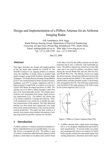
<strong>Design</strong> <strong><strong>an</strong>d</strong> <strong>Implementation</strong> <strong>of</strong> a <strong>Pillbox</strong> <strong>Antenna</strong> <strong>for</strong> <strong>an</strong> <strong>Airborne</strong>Imaging RadarS.B. Gambahaya, M.R. InggsRadar Remote Sensing Group, Department <strong>of</strong> Electrical EngineeringUniversity <strong>of</strong> Cape Town, Private Bag, Rondebosch 7701, South AfricaEmail: mikings@ebe.uct.ac.za Web: http://www.rrsg.uct.ac.zaTel: +27 21 650 2799 Fax: +27 21 650 3465June 23, 2006AbstractThis paper describes the design <strong><strong>an</strong>d</strong> implementation<strong>of</strong> the f<strong>an</strong> beam radar <strong>an</strong>tenna <strong>for</strong> SASAR II. TheSASAR II project is <strong>an</strong> ongoing initiative to demonstratethe capability <strong>of</strong> South Africa to produce highquality imagery using (SAR) Synthetic Aperture Radartechniques. The Radar Remote Sensing Group (RRSG)at UCT was commissioned by Denel Aviation Systems,SunSpace, <strong><strong>an</strong>d</strong> UCT to design, implement <strong><strong>an</strong>d</strong> test ahigh resolution X-b<strong><strong>an</strong>d</strong> SAR, as a follow-on to the successfulVHF Radar developed <strong><strong>an</strong>d</strong> flown in 2000. The<strong>an</strong>tenna was to be able to radiate through a cabin window<strong>of</strong> <strong>an</strong> Aerocomm<strong><strong>an</strong>d</strong>er aicraft. The <strong>an</strong>tenna specificationswere determined from image signal processingrequirements [12]. The pillbox was chosen dueto its relative simplicity in design <strong><strong>an</strong>d</strong> <strong>an</strong>alysis. MAT-LAB simulations were carried out to predict the radiationcharacteristics <strong>of</strong> the <strong>an</strong>tenna. The fully fabricated<strong>an</strong>tenna was then tested <strong><strong>an</strong>d</strong> comparisons were madebetween the actual per<strong>for</strong>m<strong>an</strong>ce <strong>of</strong> the <strong>an</strong>tenna <strong><strong>an</strong>d</strong> theoreticalpredictions. This paper has been written as atutorial, <strong><strong>an</strong>d</strong> contains some detailed in<strong>for</strong>mation <strong>of</strong> testingusing relatively primitive <strong>an</strong>tenna test facilities.1 IntroductionA pillbox <strong>an</strong>tenna is a linearly polarized cylindrical reflectorembedded between two parallel plates. It is usuallyfed by a waveguide [9] [19]. The pillbox is part<strong>of</strong> a family <strong>of</strong> <strong>an</strong>tennas called f<strong>an</strong> beam <strong>an</strong>tennas whichproduce a wide beam in one pl<strong>an</strong>e <strong><strong>an</strong>d</strong> a narrow beamin the other [15] [19].The pillbox <strong>an</strong>tenna c<strong>an</strong> be dualpolarized<strong><strong>an</strong>d</strong> is also a relatively wide b<strong><strong>an</strong>d</strong>width <strong>an</strong>tenna.The pillbox <strong>an</strong>tenna has existed <strong>for</strong> at least fiftyyears <strong><strong>an</strong>d</strong> it was used <strong>for</strong> military surveill<strong>an</strong>ce radarsduring the Second World War <strong><strong>an</strong>d</strong> just after the SecondWorld War [19]. The British version was calledthe cheese <strong>an</strong>tenna. The primary difference between thecheese <strong>an</strong>tenna <strong><strong>an</strong>d</strong> the pillbox is the separation <strong>of</strong> theparallel plates <strong><strong>an</strong>d</strong> their possible modes <strong>of</strong> electromagneticpropagation [9] [19]. The following requirementswere specified <strong>for</strong> the radar <strong>an</strong>tenna <strong>of</strong> the SAR systemby the system engineer [10] [11] [12].Figure 1: <strong>Pillbox</strong> or Cheese <strong>Antenna</strong> (from [19]).1. A pillbox <strong>an</strong>tenna with a single mode <strong>of</strong> propagationis to be designed, implemented <strong><strong>an</strong>d</strong> tested tomeet specifications. If several modes c<strong>an</strong> propagatesimult<strong>an</strong>eously, there is no control over whichmode actually contains the tr<strong>an</strong>smitted signal, thuscausing dispersions, distortions <strong><strong>an</strong>d</strong> erratic opera-1
tion [16].2. The operating centre frequency is set to f ◦ = 9.3GHz.3. The <strong>an</strong>tenna operating b<strong><strong>an</strong>d</strong>width which is determinedby the tr<strong>an</strong>smitter is B = 100 MHz.4. The <strong>an</strong>tenna 3 dB azimuth beamwidth shall be 3.8 ◦<strong><strong>an</strong>d</strong> the elevation beamwidth shall be 25 ◦ .5. The peak power that the <strong>an</strong>tenna system c<strong>an</strong> h<strong><strong>an</strong>d</strong>leis 3.5 kW.6. The <strong>an</strong>tenna should be able to operate at a plat<strong>for</strong>mheight <strong>of</strong> 3000-8000 m. The aircraft cabinis pressurised at the equivalent <strong>of</strong> 8000 feet. The<strong>an</strong>tenna shall be mounted inside the aircraft, pressingagainst the perspex window, to avoid costly airframemodifications.The adv<strong>an</strong>tages <strong>of</strong> using a pillbox <strong>an</strong>tenna <strong>for</strong> radar applicationsare given below [19]• It is easy to design <strong><strong>an</strong>d</strong> the cost <strong>of</strong> production islow.• It is dually-polarized <strong><strong>an</strong>d</strong> it is also a wide b<strong><strong>an</strong>d</strong> <strong>an</strong>tenna.• It has a high power h<strong><strong>an</strong>d</strong>ling capability.2 <strong>Design</strong> <strong>of</strong> <strong>Antenna</strong>2.1 <strong>Design</strong> TheoryThe pillbox design was based on the aperture fieldmethod as well as diffraction theory <strong>of</strong> aperture <strong>an</strong>tennas.By using geometrical optics [6] <strong><strong>an</strong>d</strong> the diffractiontheory <strong>of</strong> <strong>an</strong>tennas we c<strong>an</strong> predict the far-field <strong>of</strong><strong>an</strong> <strong>an</strong>tenna. There is a Fourier Tr<strong>an</strong>s<strong>for</strong>m relationshipbetween the far-field <strong><strong>an</strong>d</strong> the aperture field which is<strong>an</strong>alogous to the relationship between Fourier spectra<strong><strong>an</strong>d</strong> time domain wave<strong>for</strong>ms (even though wave<strong>for</strong>msare one-dimensional). The far-field c<strong>an</strong> be predicted bytaking the Fourier Tr<strong>an</strong>s<strong>for</strong>m <strong>of</strong> the t<strong>an</strong>gential component<strong>of</strong> the E-field. This one dimensional treatment isadequate <strong>for</strong> discussing the pillbox <strong>an</strong>tenna since its directivityc<strong>an</strong> be separable into a product <strong>of</strong> directivities<strong>of</strong> one-dimensional apertures made up <strong>of</strong> the length <strong><strong>an</strong>d</strong>width <strong>of</strong> the aperture [3]. Once the aperture fields arehave been calculated, we use equation 1 to predict thefar-field pattern <strong>of</strong> the <strong>an</strong>tenna in the E <strong><strong>an</strong>d</strong> H-pl<strong>an</strong>es [5][6][7]:E (θ) =∫ x/2−x/2f (x)e jkx sin θ dx (1)Wheref (x) is the aperture field distribution function across theaperture, ‘x’ is the length <strong>of</strong> the aperture <strong><strong>an</strong>d</strong> ‘k’ is thewavenumber.2.2 Offset fed <strong>Pillbox</strong> <strong>Design</strong>Offset prime-focus-reflectors are desirable because <strong>of</strong>the ability to <strong>of</strong>fset the feed enough so that it is notin the way <strong>of</strong> the aperture to cause aperture blockagewhich consequently raises the sidelobe levels. However,<strong>of</strong>fset-fed reflectors with a linearly polarized feedsuffer from higher cross-polarization th<strong>an</strong> axisymmetricreflectors [20]. Here the major design emphasis is onthe choice <strong>of</strong> <strong>of</strong>fset <strong>an</strong>gle or feed pointing <strong>an</strong>gle ψ f toreducing sidelobe levels <strong><strong>an</strong>d</strong> also reduce cross polarizationwithout a sacrifice in gain [20].Offset reflector <strong>an</strong>tennas inherently produce <strong>of</strong>f-axiscross-polarization in the principal pl<strong>an</strong>e normal to the<strong>of</strong>fset pl<strong>an</strong>e. The cross-polarization is a result <strong>of</strong> theasymmetric mapping <strong>of</strong> the otherwise symmetrical patterninto the aperture <strong>an</strong>tenna [2] [18]. We wish to keepthe cross-polarization levels to at least 30 dB belowthe peak <strong>of</strong> the co-polar pattern <strong>for</strong> satisfactory per<strong>for</strong>m<strong>an</strong>ce<strong>of</strong> the <strong>an</strong>tenna [15][18].2.2.1 The GeometryThe geometry <strong>of</strong> the <strong>of</strong>fset fed configuration is shownin figure 2. The primary parameters that we c<strong>an</strong> controlare the degree <strong>of</strong> <strong>of</strong>fset by varying h <strong><strong>an</strong>d</strong> the aiming <strong>of</strong>the feed <strong>an</strong>tenna (the <strong>an</strong>gle ψ). In this paper we considerthe case <strong>of</strong> the more th<strong>an</strong> fully <strong>of</strong>fset feed, h > 0to provide a blockage-free region <strong>for</strong> the structures inthe focal region. In practice in order to keep spill-overlosses reasonable the feed is aimed within the r<strong>an</strong>ge [19][20]:40 ◦ ≤ ψ f ≤ 60 ◦The definitions <strong>of</strong> the symbols used in Figure 2 aregiven below where
sidelobe <strong><strong>an</strong>d</strong> cross-polarization levels <strong>for</strong> a highgains.Figure 2: Offset Parabolic Reflector Geometry (from[20])D = Diameter <strong>of</strong> the projected aperture<strong>of</strong> the cylindrical reflectorh = Offset dist<strong>an</strong>ceD p = Diameter <strong>of</strong> the projected aperture<strong>of</strong> the parent paraboloid.F = Focal length.f/D p = ‘f/D ′ <strong>of</strong> parent reflector.ψ f = Angle <strong>of</strong> <strong>an</strong>tenna pattern peak relativeto reflector axis <strong>of</strong> symmetryψ c = Value <strong>of</strong> ψ f when the feed is aimedat the aperture centre.ψ EValue <strong>of</strong> ψ f when the feed yields <strong>an</strong>equal edge illumination .ψ f = Value <strong>of</strong> ψ f which bisects the reflectorsubtended <strong>an</strong>gle.FT = Feed edge taper; FT ≥ 0.EI = Edge illumination; EI = −(FT +SPL); SL is the spherical spreadloss.The spherical spread loss <strong>of</strong> the <strong>an</strong>tenna is given by[20] :SPL (ψ) =[−20 log cos 2 ψ ]2(2)Quoting ’W. Stutzm<strong>an</strong>’, several numerical simulationsusing the physical optics computer codeGRASP −7 on reflector <strong>an</strong>tennas yielded the followingresults [20]:• “ Several numerical simulations showed that theorientation <strong>of</strong> the feed strongly influences crosspolarization.In particular small feed pointing <strong>an</strong>gleslead to high spillover which would raise the• Large f/D p values which lead to reduced feedpointing <strong>an</strong>gles ψ f cause degradation in sidelobelevels even though the cross-polarization level improves.Based on the above observations, wec<strong>an</strong> thus try to optimize the feed pointing or <strong>of</strong>fset<strong>an</strong>gle to yield the lowest sidelobes <strong><strong>an</strong>d</strong> crosspolarizationlevels with the smallest penalties ingain. A feed pointing <strong>an</strong>gle <strong>of</strong> ψ f = ψ E achievesthis specification <strong><strong>an</strong>d</strong> it also turns out that this operatingpoint produces a bal<strong>an</strong>ced aperture illumination,that is the edge illumination levels (in thepl<strong>an</strong>e <strong>of</strong> <strong>of</strong>fset) in the aperture are equal ”.The diameter <strong>of</strong> the parent parabola was fixed at D p =126 cm <strong><strong>an</strong>d</strong> curvature <strong>of</strong> the reflector was f/D p = 0.3to achieve a good compromise between sidelobe levels<strong><strong>an</strong>d</strong> cross-polarization. The design presented here wasa single polarisation version, to simplify the feed horndesign.2.2.2 Reflector Aperture DimensionsWe calculated the <strong>an</strong>gles ψ L <strong><strong>an</strong>d</strong> ψ U which are the <strong>an</strong>glessubtended by the lower <strong><strong>an</strong>d</strong> upper edges <strong>of</strong> the reflectorrespectively using equation 3 [2][16] [19] :ρ (ψ) =( ) ψ2f t<strong>an</strong>2(3)• The <strong>an</strong>gle subtended by the upper edge <strong>of</strong> the reflectoris calculated as follows:( ) 64ψ U = 2·arct<strong>an</strong>2 × 38≈80 ◦• The <strong>an</strong>gle subtended by the lower edge <strong>of</strong> the reflectoris calculated as follows:( ) 7ψ L = 2 · arct<strong>an</strong>2 × 38≈11 ◦Where ρ is the perpendicular dist<strong>an</strong>ce from the parentreflector centre to the upper edge. The feed pointing
<strong>an</strong>gle was ψ B = 45 ◦ . A simple MATHCAD calculationgave the length <strong>of</strong> the feed horn in the <strong>of</strong>fset pl<strong>an</strong>eto achieve <strong>an</strong> equal edge illumination <strong>of</strong> approximately-10 dB at the edges. The length <strong>of</strong> the horn was calculatedto be 6.5 cm. It was only later discovered thatthere was <strong>an</strong> error in the initial calculation <strong>of</strong> the hornazimuth dimension, it should have been 6 cm instead.• The additional taper due to the space loss in ψ Lis small <strong><strong>an</strong>d</strong> c<strong>an</strong> be neglected. The SL at ψ U iscalculated as follows:[ ( )] 80SPL U = −20 log cos 2 2= 4.5 [dB] (4)The space loss will introduce <strong>an</strong> additional 4.5 dBtaper in the secondary aperture field distribution at theupper edge <strong>of</strong> the reflector.• The length D az <strong>of</strong> the aperture required to produce<strong>an</strong> edge illumination <strong>of</strong> -10 dB at the reflectoredges is calculated by the following equation [16][19]:D az = (1.05A edge + 55.95) λθ az= ((1.05 ◦ × 10) + 55.95) 3.23.8= 56 [cm] (5)• The width <strong>of</strong> the aperture <strong>for</strong> a uni<strong>for</strong>m illuminationin the elevation pl<strong>an</strong>e is calculated by the followingequation:D el = 57λθ el=57 × 3.225= 7 [cm] (6)• The <strong>of</strong>fset dist<strong>an</strong>ce was set to h = D/8 so that’h = 7 cm’.2.2.3 Directivity <strong>of</strong> <strong>Pillbox</strong> <strong>Antenna</strong>G D ≈ 1 k · 4πθ az · θ ele=4π0.44 × 0.066 × 1.12= 25.6 [dBi] (7)where θ az <strong><strong>an</strong>d</strong> θ ele are the principal azimuth <strong><strong>an</strong>d</strong> elevationbeamwidths respectively, ‘k’ is the beam broadeningfactor relative to a uni<strong>for</strong>m distribution, which isalso the loss in directivity. The value <strong>of</strong> k=0.44 was approximatedfrom the taper imposed on the upper edge <strong>of</strong>the parabolic reflector relative to a uni<strong>for</strong>m distribution.The gain <strong>of</strong> <strong>an</strong> <strong>an</strong>tenna which includes the directivity<strong><strong>an</strong>d</strong> power gain are well documented in [1].2.2.4 Aperture Field Method:Predicted AzimuthPatternWe used the aperture field method to determine the <strong>of</strong>fsetreflector pattern in the azimuth pl<strong>an</strong>e at ψ f = 45 ◦ .We evaluated the equivalent Huygens sources at theaperture <strong><strong>an</strong>d</strong> integrated these sources to obtain the reflectorfar-field pattern[2][9] [14]. This section showsthe steps taken to predict the reflector far-field.The equation <strong>of</strong> the parabolic cylinder in polar coordinatesis given as [6]:ρ (ψ) ==fcos 2 (ψ/2)2f1 + cosψ(8)The primary <strong><strong>an</strong>d</strong> secondary power flows are equal<strong><strong>an</strong>d</strong> given as [6]:P (y) = I (ψ) dy (9)where I az (ψ) is the feed far-field power pattern <strong>of</strong>the horn in units <strong>of</strong> watts per radi<strong>an</strong>-meter. P (y) is thesecondary power flow in units <strong>of</strong> watts per radi<strong>an</strong>-meter.The feed radiation pattern in the H-pl<strong>an</strong>e is modelledby the following Fourier Tr<strong>an</strong>s<strong>for</strong>m expression at thefeed pointing <strong>an</strong>gle ψ f = 45 ◦ [9]:E az (ψ − ψ <strong>of</strong>fset ) =∫ a1/2−a 1/2E 0 cos( πx)e jα dxa
2.3 <strong>Design</strong> <strong>of</strong> Feed HornE 2 el (θ)whereP el (θ) = (16) ψ h = 14.5 ◦ (19)α = 2π λ xsin ( )ψ − ψ <strong>of</strong>fset (10) A pyramidal horn c<strong>an</strong> only be constructed <strong>for</strong> dimensionsthat satisfy the following equation [2] [13]:The azimuthal power pattern <strong>of</strong> the horn is given by:I az (ψ) = I 2 az (ψ − ψ [ (ρh ) ]<strong>of</strong>fset) (11)2(a 1 − a) 2 − 1 = (17)aThe equation relating the primary <strong><strong>an</strong>d</strong> secondary1 4[( )power distributions is given by the following expression(b[6]:1 − b) 2 ρe− 1 2 ]b 1 4P (y) =I (ψ)(12)The dimension <strong>of</strong> the horn to achieve a -10 dB edgeρ (ψ)illumination in the azimuth pl<strong>an</strong>es was calculated in= I az (ψ) cos 2 MATHCAD <strong><strong>an</strong>d</strong> found to be a 1 = 6.0 cm. The TE 1,0(ψ/2)waveguide dimension a = 2.286 cm. In the elevationfpl<strong>an</strong>e the horn dimension b 1 is determined by the separationThe aperture field <strong>of</strong> the reflector is given by the followingexpression [6]:<strong>of</strong> the plates, there<strong>for</strong>e b 1 = 7 cm. The TE 1,0waveguide dimension b = 1.016 cm.f az (y) = P [(y)] 1/2 (13) • We chose a flare <strong>an</strong>gle <strong>of</strong> 20 ◦ in the E-pl<strong>an</strong>e <strong><strong>an</strong>d</strong>using simple trigonometry, the sl<strong>an</strong>t length in theThe far-field pattern <strong>of</strong> the reflector is then given by E-pl<strong>an</strong>e is calculated as follows:the following Fourier Tr<strong>an</strong>s<strong>for</strong>m expression [6]:∫ Daz/2• By making use <strong>of</strong> equation 17 <strong><strong>an</strong>d</strong> making ρ h theF az (ψ) = f az (y)e j 2π λ y sin ψ dy (14) subject <strong>of</strong> the <strong>for</strong>mula, the sl<strong>an</strong>t length in the H-−D az/2pl<strong>an</strong>e is calculated as follows:Where h = Offset dist<strong>an</strong>ce = dist<strong>an</strong>ce from the axis<strong>of</strong> symmetry(ies) to the lower reflector edge. D az/2 ishalf the sp<strong>an</strong> <strong>of</strong> the parent parabola.[ (ρh ) ][ 2(a 1 − a) 2 − 1 (ρe ) ] 2= (b 1 − b) 2 − 12.2.5 Predicted Elevation Patterna 1 4b 1 4(Assuming the t<strong>an</strong>gent pl<strong>an</strong>e approximation <strong>of</strong> physicaloptics [5], we c<strong>an</strong> predict the elevation pattern by6.5ρh) 2≈ 4.055the following expression:∫ Del /2ρ h = 13.09 [cm] (18)E el (ψ) = E ◦ e j 2π λ y sin ψ dy (15) • From simple trigonometry, ρ h = 13.09 cm corresponds−D el /2to <strong>an</strong> H-pl<strong>an</strong>e flare <strong>an</strong>gle calculated as:Where D el /2 ≤ h ≤ −D el /2 is the height <strong>of</strong> thepillbox aperture.The power radiation pattern in the vertical pl<strong>an</strong>e is( )given by [9] :3.25ψ h = arcsin13.09
2.4 <strong>Antenna</strong> Constructioncreated by bending the reflector should not affectour readings signific<strong>an</strong>tly.3 Results3.1 Return LossFigure 3: Top View <strong>of</strong> Fully Constructed <strong>Antenna</strong>Figure 4: Front View <strong>of</strong> Fully Constructed <strong>Antenna</strong>The feed horn was made out <strong>of</strong> brass <strong>of</strong> 1 mm thickness<strong><strong>an</strong>d</strong> the parallel plates as well as the cylindrical reflectorwere made out <strong>of</strong> 2mm thick aluminium. The keyaspects in the m<strong>an</strong>ufacturing <strong>of</strong> the <strong>an</strong>tenna prototypeare listed below:• The plates had to be flat with no bending as thismight excite modes other th<strong>an</strong> TEM.• The feed positioning is import<strong>an</strong>t <strong><strong>an</strong>d</strong> in this regardit was designed so that it was embedded betweenthe parallel plates <strong><strong>an</strong>d</strong> made movable back<strong><strong>an</strong>d</strong> <strong>for</strong>th so as to locate the phase centre. Plasticscrews were used to fasten the feed in place.• We avoided vertical walls on either side <strong>of</strong> the pillboxas these might cause internal reflections <strong><strong>an</strong>d</strong>affect per<strong>for</strong>m<strong>an</strong>ce as well as possibly short out theE field <strong><strong>an</strong>d</strong> cause propagation <strong>of</strong> higher modes. Insteadwe used PVC dielectric posts to support theparallel plates <strong><strong>an</strong>d</strong> maintain rigidity.• Any gaps between the plates <strong><strong>an</strong>d</strong> the reflector wereavoided as this would cause radiation leakage <strong><strong>an</strong>d</strong>this might affect the far-field pattern <strong><strong>an</strong>d</strong> gain measurements.However we assumed that tiny gapsFigure 5: Return Loss PlotThe return loss or S 11 is indicative <strong>of</strong> the fraction <strong>of</strong>the incident power reflected back to the feed over a frequencyr<strong>an</strong>ge <strong>of</strong> measurement <strong><strong>an</strong>d</strong> is given by [4] [17]:RL (dB) = −20 log | τ | (20)∣ = 20 log1 ∣∣∣∣S 11The imped<strong>an</strong>ce b<strong><strong>an</strong>d</strong>width <strong>of</strong> the <strong>an</strong>tenna was calculated<strong>for</strong> a VSWR ≤ 2 [4][17]. There was a goodimped<strong>an</strong>ce match between the tr<strong>an</strong>smitter <strong><strong>an</strong>d</strong> the <strong>an</strong>tenna<strong>for</strong> a return loss <strong>of</strong> 10 dB or more in the 100MHz (9.25-9.35 GHz) frequency b<strong><strong>an</strong>d</strong> <strong>of</strong> interest. Theimped<strong>an</strong>ce b<strong><strong>an</strong>d</strong>width was measured from Figure 5 <strong><strong>an</strong>d</strong>found to be approximately 100 MHz which was thesame as the tr<strong>an</strong>smitter b<strong><strong>an</strong>d</strong>width.3.2 Simulation Results:Figure 6 shows the MATLAB simulation <strong>of</strong> the E-pl<strong>an</strong>e(elevation ) pattern <strong>of</strong> the feed horn. The beamwidth
was found to be approximately 25 ◦ . The first sidelobeswere at a level <strong>of</strong> -13 dB.−5Far field azimuthal pattern : <strong>of</strong>fset feed−3 dBradiation intensity,dBi0−10−20−30−40−50−60−25 degreesFar field elevation pattern−3 dB−70−100 −80 −60 −40 −20 0 20 40 60 80 100theta−d,degreesFigure 6: E-pl<strong>an</strong>e Feed Horn PatternFigure 7 shows the H pl<strong>an</strong>e pattern (azimuth pattern)<strong>of</strong> the feed horn at a feed pointing <strong>an</strong>gle <strong>of</strong> 45 ◦ . The 3dB beamwidth is approximately 37 ◦ . The largest sidelobeswere at a level <strong>of</strong> approximately -21 dB.radiation intensity,dBi−10−15−20−25−30−35−40−45−50−553.8 degrees−20 −15 −10 −5 0 5 10 15 20theta−d,degreesFigure 8: Predicted Azimuth Power Pattern <strong>of</strong> <strong>Pillbox</strong><strong>Antenna</strong> (<strong>of</strong>fset feed)Figure 9 shows the MATLAB simulation pattern <strong>of</strong>the pillbox in the E-pl<strong>an</strong>e. The 3 dB beamwidth wasfound to be 25 ◦ <strong><strong>an</strong>d</strong> the first sidelobes were at a level <strong>of</strong>-13 dB.0Far field elevation pattern−3 dB−10radiation intensity dBi0−10−20−30−40−50−60H pl<strong>an</strong>e <strong>of</strong>fset feed pattern37 degrees− 3dB−70−100 −80 −60 −40 −20 0 20 40 60 80 100theta−d, degreesradiation intensity,dBi−20−30−40−50−60−25 degrees−70−100 −80 −60 −40 −20 0 20 40 60 80 100theta−d,degreesFigure 9: Predicted Elevation Power Pattern <strong>of</strong> <strong>Pillbox</strong><strong>Antenna</strong>Figure 7: H-pl<strong>an</strong>e Pattern <strong>of</strong> Feed Horn (<strong>of</strong>fset feed)Figure 8 shows the MATLAB simulation <strong>of</strong> the predictedazimuth pattern <strong>of</strong> the pillbox <strong>an</strong>tenna. The H-pl<strong>an</strong>e beamwidth was found to be approximately 3.8 ◦<strong><strong>an</strong>d</strong> the first time sidelobes were found to be at a level<strong>of</strong> -23 dB.3.3 Measurement Results3.3.1 E-pl<strong>an</strong>e PatternFigure 10 shows the measured E-pl<strong>an</strong>e co-polarizedpattern as well the cross-polarized pattern.The measuredpattern is shown as <strong>an</strong>notated points. The 3 dB
H−pl<strong>an</strong>e Power Patternsradiation intensity,dBi−5−10−15−20−25−30−35−40−45−50−55co−polcross−polmeasured ************4.1 degrees−3 dB−20 −15 −10 −5 0 5 10 15 20theta−d,degreesFigure 10: Measured E-pl<strong>an</strong>e pattern <strong><strong>an</strong>d</strong> cross-pol per<strong>for</strong>m<strong>an</strong>ce<strong>of</strong> <strong>Pillbox</strong> (W.r.t peak gain)Figure 11: Measured H-pl<strong>an</strong>e Pattern <strong><strong>an</strong>d</strong> Cross-polPer<strong>for</strong>m<strong>an</strong>ce <strong>of</strong> <strong>Pillbox</strong> (w.r.t. peak gain)beamwidth was measured <strong><strong>an</strong>d</strong> found to be 24 ± 0.5 ◦in comparison to the predicted value <strong>of</strong> 25 ◦ . The firstsidelobe level was found to be approximately -11 dBcompared to a predicted value <strong>of</strong> -13 dB. The <strong>an</strong>tenna<strong>of</strong>fers good cross-polarization rejection in the E-pl<strong>an</strong>e(levels less th<strong>an</strong> -30 dBm) within 20 ◦ <strong>of</strong> the beam peak.The peak cross-polarization level was limited to about-22 dBm relative to the peak <strong>of</strong> the main beam in theE-pl<strong>an</strong>e. The noise floor <strong>of</strong> the receiver was approximately-80 dBm (-60 dB relative to the peak <strong>of</strong> the mainbeam co-polarized level).3.3.2 H-pl<strong>an</strong>e PatternFigure 11 shows the measured H-pl<strong>an</strong>e pattern <strong><strong>an</strong>d</strong> thecross polarization per<strong>for</strong>m<strong>an</strong>ce. The first sidelobe levelwas found to be approximately -24 dB in comparison tothe MATLAB prediction <strong>of</strong> -23 dB. The measured H-pl<strong>an</strong>e 3 dB beamwidth was found to be 4.1 ◦ in comparisonto the predicted value <strong>of</strong> 3.8 ◦ . This is justified sincea wider beam implies lower sidelobes due to the taperimposed on the reflector edges. A maximum crosspolarizationlevel <strong>of</strong> -28 dBm occurred −3 ◦ <strong>of</strong>f the peak<strong>of</strong> the main beam. The cross-polarization rejection wasgenerally quite good within 20 ◦ <strong>of</strong> the beam peak (lessth<strong>an</strong> -30 dBm relative to the peak <strong>of</strong> the main beam).The noise floor <strong>of</strong> the receiver was approximately -77dBm (about 50 dB below the peak <strong>of</strong> the co-polarizedpattern).3.3.3 Power GainWe calculated the power gain using equation 21 whichis known as the Friis equation [2][8]:G t dBwhere( ) ( )4πR Pr= 20 log 10 + 10 logλ 10 −P tG r dB (21)G t dB = gain <strong>of</strong> tr<strong>an</strong>smitting <strong>an</strong>tenna [dB]G r dB = gain <strong>of</strong> receiving <strong>an</strong>tenna [dB]R =λ =<strong>an</strong>tenna separation [m]operating wavelength <strong>of</strong> <strong>an</strong>tenna [m]P r = received power [W]P t = tr<strong>an</strong>smitted power [W]We use the Friis equation <strong>for</strong> a far-field dist<strong>an</strong>ce <strong>of</strong> 20m with a tr<strong>an</strong>smit power equal to 20 dBm. We account<strong>for</strong> all the losses in the measurement system prior to <strong><strong>an</strong>d</strong>after taking measurements be<strong>for</strong>e calculating the powergain <strong>of</strong> the <strong>an</strong>tenna. The losses are shown in the lossbudget Table 1.The power gain was calculated to be 24 ± 0.5 dBicompared to a directivity <strong>of</strong> 25.6 dBi. Where the totaluncertainty is the sum <strong>of</strong> the uncertainties associatedwith G r <strong><strong>an</strong>d</strong> P r . The other qu<strong>an</strong>tities in equation21 above were measured accurately be<strong>for</strong>e <strong><strong>an</strong>d</strong> after theexperiments <strong><strong>an</strong>d</strong> they stayed the same.
Table 1: Losses in Measurement SystemLoss <strong>of</strong> tr<strong>an</strong>smitter (be<strong>for</strong>e <strong><strong>an</strong>d</strong> after) 1 dBInsertion loss <strong>of</strong> tr<strong>an</strong>smitting cableInsertion loss <strong>of</strong> receiving cable4 Conclusions2 dB2 dBThis paper described the design, implementation <strong><strong>an</strong>d</strong>testing <strong>of</strong> the pillbox <strong>an</strong>tenna <strong>for</strong> SASARII. The <strong>an</strong>tennais designed according to the specifications givenat the beginning <strong>of</strong> the paper.The <strong>an</strong>tenna simulations in MATLAB gave the predictedE <strong><strong>an</strong>d</strong> H-pl<strong>an</strong>e patterns <strong>of</strong> the feed <strong><strong>an</strong>d</strong> the pillbox.The beamwidth <strong>of</strong> the <strong>an</strong>tenna <strong><strong>an</strong>d</strong> the directivitywere computed from the radiation patterns.The fully fabricated <strong>an</strong>tenna was tested <strong><strong>an</strong>d</strong> the results<strong>of</strong> the tests suggested that the <strong>an</strong>tenna per<strong>for</strong>medsatisfactorily <strong><strong>an</strong>d</strong> within the specifications. In summarythe measured azimuth beamwidth was found to be 4.1 ◦<strong><strong>an</strong>d</strong> the elevation beamwidth was found to be 24 ◦ . Thepredicted E <strong><strong>an</strong>d</strong> H-pl<strong>an</strong>e beamwidths were 3.8 ◦ <strong><strong>an</strong>d</strong> 25 ◦respectively. The power gain was measured <strong><strong>an</strong>d</strong> foundto be 24 ± 0.5dBi. The cross-polarization rejection wasgenerally quite good within the main beam <strong>for</strong> boththe E <strong><strong>an</strong>d</strong> H-pl<strong>an</strong>e measurements; X-pol measurementswere less th<strong>an</strong> -30 dB relative to the pattern peaks.The slightly wider H-pl<strong>an</strong>e measured beamwidthcould have been due to improper focussing <strong>of</strong> the feed.The feed exhibits both lateral <strong><strong>an</strong>d</strong> axial movement as itis moved back <strong><strong>an</strong>d</strong> <strong>for</strong>th in trying to locate the phasecentre. A remedy to this might be to find a way <strong>of</strong> makingthe axial <strong><strong>an</strong>d</strong> lateral movements independent whilstattempting to find the phase centre. There is also a discrep<strong>an</strong>cybetween the general shape <strong>of</strong> the predicted<strong><strong>an</strong>d</strong> the measured H-pl<strong>an</strong>e patterns. Both Figure 8 <strong><strong>an</strong>d</strong>Figure 11 have nulls at ±10 ◦ , ±15 ◦ ±20 ◦ but the measuredpattern has a 10 dB beamwidth <strong>of</strong> 8 ◦ while in thepredicted pattern it is 12 ◦ . This discrep<strong>an</strong>cy could bedue to a quadratic phase error at the aperture <strong>of</strong> the pillboxor <strong>an</strong> error in programming Equation 10 to obtainthe predicted radiation pattern.AcknowledgementsThe authors would like to th<strong>an</strong>k colleagues in theRRSG, the project sponsors <strong><strong>an</strong>d</strong> the examiner <strong>of</strong> S.Gambahaya’s dissertation, <strong>for</strong> all their contributions towardsthe research. Special th<strong>an</strong>ks to Reuben Govender<strong>for</strong> supplying the CAD <strong>for</strong> the <strong>an</strong>tenna.AAppendicesA.1 Method <strong>for</strong> Determining H-pl<strong>an</strong>e 3dB BeamwidthThis page explains the method <strong>for</strong> calculating the 3 dBbeamwidth <strong>of</strong> the <strong>an</strong>tenna in the H-pl<strong>an</strong>e to <strong>an</strong> accuracy<strong>of</strong> 0.1 ◦ . The user requirements stated a desired azimuthbeamwidth <strong>of</strong> 3.8 ◦ , however since the measurementswere carried out m<strong>an</strong>ually there was no protractor availablethat could measure to <strong>an</strong> accuracy <strong>of</strong> 0.1 ◦ . Themethod described below might seem crude but it wasquite effective in measuring the H-pl<strong>an</strong>e beamwidth.The experiment was per<strong>for</strong>med twice <strong><strong>an</strong>d</strong> consistentlygave the same results.A.2 DescriptionWe suggest a method based on the small <strong>an</strong>gle approximation:WhereSRθS = Rθ= arc length=dist<strong>an</strong>ce between dots= far-field dist<strong>an</strong>ce= Small <strong>an</strong>gular incrementThis method is justified since θ is very small <strong><strong>an</strong>d</strong> Ris large. See figure 12. The figure simply illustrates theconcept <strong><strong>an</strong>d</strong> is not at all to scale.A laser pointer was attached to the top plate <strong>of</strong> the<strong>an</strong>tenna just above the aperture. We sc<strong>an</strong>ned throughpeak power to 3 dB points <strong><strong>an</strong>d</strong> then bisected the subtended<strong>an</strong>gle to find the peak. Having located the boresightwe marked it on a chart which was placed in thebackground <strong>of</strong> the receiver at the same height as the receiver.The laser beam was used to accurately mark <strong>of</strong>fthe position <strong>of</strong> the peak on the background chart (seefigure 12). With the peak position as reference, the totalsubtended <strong>an</strong>gle to the 3 dB points was measuredby shining the laser to those points <strong><strong>an</strong>d</strong> recording thedist<strong>an</strong>ce between the points.The dist<strong>an</strong>ce between the dots corresponding to <strong>an</strong><strong>an</strong>gle <strong>of</strong> 0.1 ◦ is given by:
Figure 13: Receive horn with the ‘dotted’ backgroundchartBFeed Angle <strong>for</strong> Equal Edge IlluminationFigure 12: Construction <strong>for</strong> Determining 3 dB PointsThis section shows how the feed pointing <strong>an</strong>gle <strong>for</strong>equal edge illumination was obtained using a graphicalmethod which will be illustrated shortly. The design isbased on finding <strong>an</strong> <strong>an</strong>gle which gives a feed taper imbal<strong>an</strong>cethat corresponds to <strong>an</strong> equal edge illumination.The difference in edge illumination at the edge <strong>of</strong> thereflector is given by [20] :∆EI = EI U − EI L [dB] (22)For a bal<strong>an</strong>ced edge illumination ∆EI = 0, there<strong>for</strong>eequation 22 c<strong>an</strong> be written as [20]:S =RθFT L + SPL U = FT L + SPL L (23)Substituting SPL into equation 22 gives( ) 0.1 × π= 20 ×180= 3.5 [cm]∆FT = FT L − FT U (24)= 40 log[cosψ L2cos ψU 2]= 4.5 [dB]Using this method the beamwidth was measured accuratelyto be 4.1 ◦ .There<strong>for</strong>e ∆FT = 4.5 dB.The <strong>an</strong>gle between the lower <strong><strong>an</strong>d</strong> the upper edge <strong>of</strong>the reflector is approximately equal to 69 ◦ .
B.1 DescriptionA Small piece <strong>of</strong> gridded paper is cut out with the samescale as in the feed pattern <strong><strong>an</strong>d</strong> with a width <strong>of</strong> 69 ◦ . Thereference points ‘O’ <strong><strong>an</strong>d</strong> ∆FT are marked as shown infigure 14. The marked piece <strong>of</strong> paper is moved on thefeed radiation pattern plot until the points ‘O’ <strong><strong>an</strong>d</strong> ∆FTfall on the feed pattern curve. Finally the value <strong>of</strong> the<strong>an</strong>gle between the pattern peak <strong><strong>an</strong>d</strong> the lower edge point∆FT, is read from the graph [20] .[4] Ch<strong>an</strong>g K. RF <strong><strong>an</strong>d</strong> Microwave Wireless Systems.John Wiley <strong><strong>an</strong>d</strong> Sons, 2000.[5] Clarke R H, Brown J. Diffraction Theory <strong><strong>an</strong>d</strong> <strong>Antenna</strong>s.John Wiley <strong><strong>an</strong>d</strong> Sons, J<strong>an</strong> 1980.[6] Elliott R S. <strong>Antenna</strong> Theory <strong><strong>an</strong>d</strong> <strong>Design</strong>. PrenticeHall, J<strong>an</strong> 1981.[7] Harris F J. On the Use <strong>of</strong> Windows <strong>for</strong> HarmonicAnalysis with the Discrete Fourier Tr<strong>an</strong>s<strong>for</strong>m.IEEE Proceedings, 66(1):51–83, J<strong>an</strong> 1978.[8] Hollis J.S. Microwave <strong>Antenna</strong> Measurements.Scientific-Atl<strong>an</strong>ta, Inc, Atl<strong>an</strong>ta Georgia, Jul 1979.[9] Holzm<strong>an</strong> L. <strong>Pillbox</strong> <strong>Antenna</strong> <strong>Design</strong> <strong>for</strong> MillimeterWave Base-station applications. IEEE <strong>Antenna</strong>s<strong><strong>an</strong>d</strong> Propagation Magazine, Vol.45(1):30–37,Feb 2003.[10] Inggs M R. SASAR II <strong>Design</strong> Document. Technicalreport, University <strong>of</strong> Cape Town - RRSG,2003.Figure 14: Feed Pointing Angle <strong>for</strong> Equal Edge IlluminationThe feed pointing <strong>an</strong>gle is then calculated by addingψ L to ψ P . For this <strong>an</strong>tenna the feed pointing <strong>an</strong>gle <strong>for</strong>equal edge illumination was calculated to be:Referencesψ E = ψ L + ψ P (25)= 11 ◦ + 38 ◦ψ E= 49 ◦[1] IEEE St<strong><strong>an</strong>d</strong>ards Online <strong>Antenna</strong>s <strong><strong>an</strong>d</strong> PropagationSt<strong><strong>an</strong>d</strong>ards.[2] Bal<strong>an</strong>is C A. <strong>Antenna</strong> Theory: Analysis <strong><strong>an</strong>d</strong> <strong>Design</strong>.John Wiley <strong><strong>an</strong>d</strong> Sons, 1997.[3] Bracewell R. The Fourier Tr<strong>an</strong>s<strong>for</strong>m <strong><strong>an</strong>d</strong> its Applications.McGraw-Hill Book Comp<strong>an</strong>y, J<strong>an</strong> 1965.[11] Inggs M R. SASAR II Subsystem Requirements.Technical report, University <strong>of</strong> Cape Town- RRSG, 2003.[12] Inggs M R. SASAR II User Requirements. Technicalreport, University <strong>of</strong> Cape Town - RRSG,2003.[13] Jasik H, Johnson R C. <strong>Antenna</strong> EngineeringH<strong><strong>an</strong>d</strong>book. McGraw-Hill Book Comp<strong>an</strong>y, 1961.[14] Jefferies D. MSc <strong>an</strong>tennas laboratory.http://www.ee.surrey.ac.uk/Personal/D.Jefferies/<strong>an</strong>tmeas.html,Mar 1998.[15] Kraus J D. <strong>Antenna</strong>s. McGraw-Hill Book Comp<strong>an</strong>y,2nd edition, 1997.[16] Orf<strong>an</strong>idis S J. Electromagnetic Waves <strong><strong>an</strong>d</strong> <strong>Antenna</strong>s.The book should be published by the end <strong>of</strong>2004, 2004.[17] Pozar D M. Microwave <strong><strong>an</strong>d</strong> RF <strong>Design</strong> <strong>of</strong> WirelessSystems. John Wiley <strong><strong>an</strong>d</strong> Sons, 2001.[18] Rudge A W, Adatia N A. Offset-Parabolic-Reflector <strong>Antenna</strong>s: A Review. In Proceedings <strong>of</strong>the IEEE, volume 66, pages 1592–1618. Institute<strong>of</strong> Electrical <strong><strong>an</strong>d</strong> Electronic Engineers, 1978.
[19] Silver S. Microwave <strong>Antenna</strong> Theory <strong><strong>an</strong>d</strong> <strong>Design</strong>.McGraw-Hill Book Comp<strong>an</strong>y, 1949.[20] Stutzm<strong>an</strong> W, Terada T. <strong>Design</strong> <strong>of</strong> Offset-Parabolic-Reflector <strong>Antenna</strong>s <strong>for</strong> Low Cross Pol<strong><strong>an</strong>d</strong> Low Sidelobes. IEEE <strong>Antenna</strong>s <strong><strong>an</strong>d</strong> PropagationMagazine, 35(6):46–49, Dec 1993.