multivariate production systems optimization - Stanford University

account for different flow regimes. The more recent correlations of Duns & Ros (1963),
Orkiszewski (1967), Aziz et al. (1972), and Beggs & Brill (1973) account for slippage
between the phases and provide different algorithms to model different flow regimes.
3.3 The Correlation of Hagedorn and Brown (1965)
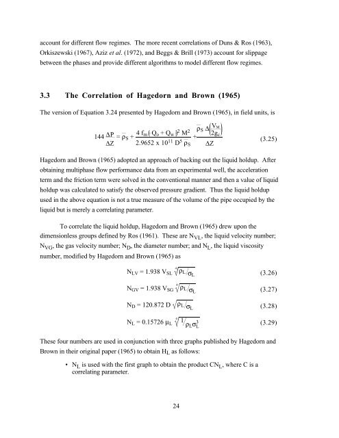
The version of Equation 3.24 presented by Hagedorn and Brown (1965), in field units, is
144 ΔP
ΔZ = ρS + 4 fm Qo + Qw 2 M2 2.9652 x 1011 D5 +
ρS
24
ρS Δ VM
ΔZ
2gc
(3.25)
Hagedorn and Brown (1965) adopted an approach of backing out the liquid holdup. After
obtaining multiphase flow performance data from an experimental well, the acceleration
term and the friction term were solved in the conventional manner and then a value of liquid
holdup was calculated to satisfy the observed pressure gradient. Thus the liquid holdup
used in the above equation is not a true measure of the volume of the pipe occupied by the
liquid but is merely a correlating parameter.
To correlate the liquid holdup, Hagedorn and Brown (1965) drew upon the
dimensionless groups defined by Ros (1961). These are NVL , the liquid velocity number;
NVG , the gas velocity number; ND , the diameter number; and NL , the liquid viscosity
number, modified by Hagedorn and Brown (1965) as
4
NLV = 1.938 VSL
ρL σL
4
NGV = 1.938 VSG
ρL σL
(3.26)
(3.27)
ND = 120.872 D ρL σL (3.28)
4
NL = 0.15726 μL
1 3
ρLσL (3.29)
These four numbers are used in conjunction with three graphs published by Hagedorn and
Brown in their original paper (1965) to obtain HL as follows:
• N L is used with the first graph to obtain the product CN L , where C is a
correlating parameter.