Solutions to the practice problems. - UCLA Biostatistics

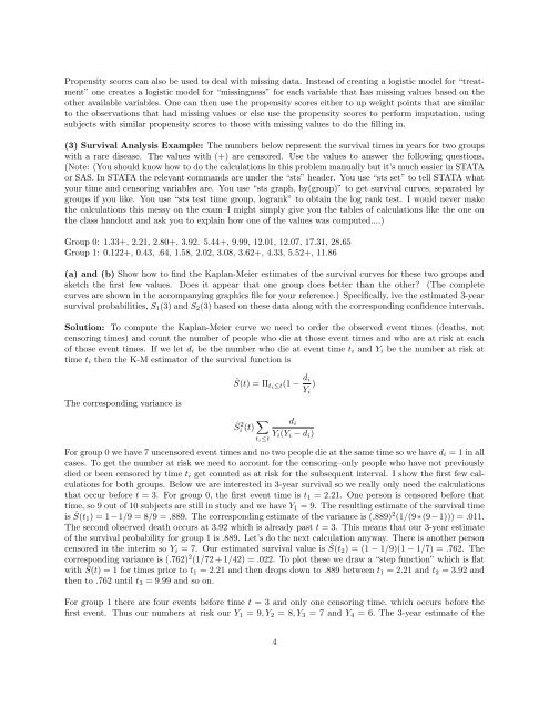
Propensity scores can also be used to deal with missing data. Instead of creating a logistic model for “treatment”
one creates a logistic model for “missingness” for each variable that has missing values based on the
other available variables. One can then use the propensity scores either to up weight points that are similar
to the observations that had missing values or else use the propensity scores to perform imputation, using
subjects with similar propensity scores to those with missing values to do the filling in.
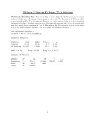
(3) Survival Analysis Example: The numbers below represent the survival times in years for two groups
with a rare disease. The values with (+) are censored. Use the values to answer the following questions.
(Note: (You should know how to do the calculations in this problem manually but it’s much easier in STATA
or SAS. In STATA the relevant commands are under the “sts” header. You use “sts set” to tell STATA what
your time and censoring variables are. You use “sts graph, by(group)” to get survival curves, separated by
groups if you like. You use “sts test time group, logrank” to obtain the log rank test. I would never make
the calculations this messy on the exam–I might simply give you the tables of calculations like the one on
the class handout and ask you to explain how one of the values was computed....)
Group 0: 1.33+, 2.21, 2.80+, 3.92. 5.44+, 9.99, 12.01, 12.07, 17.31, 28.65
Group 1: 0.122+, 0.43, .64, 1.58, 2.02, 3.08, 3.62+, 4.33, 5.52+, 11.86
(a) and (b) Show how to find the Kaplan-Meier estimates of the survival curves for these two groups and
sketch the first few values. Does it appear that one group does better than the other (The complete
curves are shown in the accompanying graphics file for your reference.) Specifically, ive the estimated 3-year
survival probabilities, S 1 (3) and S 2 (3) based on these data along with the corresponding confidence intervals.
Solution: To compute the Kaplan-Meier curve we need to order the observed event times (deaths, not
censoring times) and count the number of people who die at those event times and who are at risk at each
of those event times. If we let d i be the number who die at event time t i and Y i be the number at risk at
time t i then the K-M estimator of the survival function is
The corresponding variance is
Ŝ(t) = Π ti≤t(1 − d i
Y i
)
Ŝ 2 i (t) ∑ t i≤t
d i
Y i (Y i − d i )
For group 0 we have 7 uncensored event times and no two people die at the same time so we have d i = 1 in all
cases. To get the number at risk we need to account for the censoring–only people who have not previously
died or been censored by time t i get counted as at risk for the subsequent interval. I show the first few calculations
for both groups. Below we are interested in 3-year survival so we really only need the calculations
that occur before t = 3. For group 0, the first event time is t 1 = 2.21. One person is censored before that
time, so 9 out of 10 subjects are still in study and we have Y 1 = 9. The resulting estimate of the survival time
is Ŝ(t 1) = 1−1/9 = 8/9 = .889. The corresponding estimate of the variance is (.889) 2 (1/(9∗(9−1))) = .011.
The second observed death occurs at 3.92 which is already past t = 3. This means that our 3-year estimate
of the survival probability for group 1 is .889. Let’s do the next calculation anyway. There is another person
censored in the interim so Y i = 7. Our estimated survival value is Ŝ(t 2) = (1 − 1/9)(1 − 1/7) = .762. The
corresponding variance is (.762) 2 (1/72 + 1/42) = .022. To plot these we draw a “step function” which is flat
with Ŝ(t) = 1 for times prior to t 1 = 2.21 and then drops down to .889 between t 1 = 2.21 and t 2 = 3.92 and
then to .762 until t 3 = 9.99 and so on.
For group 1 there are four events before time t = 3 and only one censoring time, which occurs before the
first event. Thus our numbers at risk our Y 1 = 9, Y 2 = 8, Y 3 = 7 and Y 4 = 6. The 3-year estimate of the
4