Parametric and Nonparametric Linkage Analysis - Princeton University
Parametric and Nonparametric Linkage Analysis - Princeton University
Parametric and Nonparametric Linkage Analysis - Princeton University

You also want an ePaper? Increase the reach of your titles
YUMPU automatically turns print PDFs into web optimized ePapers that Google loves.
Kruglyak et al.: <strong>Parametric</strong> <strong>and</strong> <strong>Nonparametric</strong> <strong>Linkage</strong> <strong>Analysis</strong><br />
pedigree <strong>and</strong> (ii) deciding whether the inheritance information<br />
indicates the presence of a trait-causing gene.<br />
Ideally, one would like to know the precise inheritance<br />
pattern at every locus in the genome. The inheritance<br />
pattern at each point x is completely described by a<br />
binary inheritance vector v(x) = (plml Pp2,m2,<br />
... ,pn ,mn), whose coordinates describe the outcome of<br />
the paternal <strong>and</strong> maternal meioses giving rise to the n<br />
nonfounders in the pedigree (L<strong>and</strong>er <strong>and</strong> Green 1987).<br />
Specifically, pi = 0 or 1, according to whether the gr<strong>and</strong>paternal<br />
or gr<strong>and</strong>maternal allele was transmitted in the<br />
paternal meiosis giving rise to the ith nonfounder; mi<br />
carries the same information for the corresponding maternal<br />
meiosis. Thus, the inheritance vector completely<br />
specifies which of the 2f distinct founder alleles are inherited<br />
by each nonfounder. The notion of the inheritance<br />
vector is illustrated in figure 1A. The set of all 22n<br />
possible inheritance vectors will be denoted V. Similar<br />
representations of inheritance have been proposed in<br />
the context of Monte Carlo linkage analysis (Sobel <strong>and</strong><br />
Lange 1993; Thompson 1994), as well as in other applications<br />
(Whittemore <strong>and</strong> Halpern 1994a, 1994b; Guo<br />
1995).<br />
The Inheritance Distribution<br />
In practice, it is not feasible to determine the true<br />
inheritance vector at every point in the genome, since<br />
this would require genotyping all pedigree members<br />
with an infinitely dense map of fully informative markers.<br />
Because key pedigree members are frequently unavailable<br />
<strong>and</strong> genetic markers have limited heterozygosity,<br />
genotype data will provide only partial information<br />
about inheritance.<br />
Partial information extracted from a pedigree can be<br />
represented by a probability distribution over the possible<br />
inheritance vectors at each locus in the genomethat<br />
is, P(v(x) = w) for all inheritance vectors wE V. In<br />
the absence of any genotype information, all inheritance<br />
vectors are equally likely according to Mendel's first<br />
law, <strong>and</strong> the probability distribution is uniform (abbreviated<br />
as Puniform). As genotype information is added,<br />
the probability distribution is concentrated on certain<br />
inheritance vectors. The probability distribution over<br />
possible inheritance vectors will be referred to as the<br />
inheritance distribution; the notion is illustrated in figure<br />
1B <strong>and</strong> C.<br />
Calculating the Inheritance Distribution by Use of<br />
Hidden Markov Models (HMMs)<br />
To extract the full information from a data set, one<br />
must calculate the inheritance distribution conditional<br />
on the genotypes at all marker loci (abbreviated<br />
Pcomplete). L<strong>and</strong>er <strong>and</strong> Green (1987) described how, in<br />
principle, an HMM can be used to solve this problem.<br />
In brief, the approach considers the inheritance pattern<br />
a<br />
A.<br />
C.<br />
[xl,x2] [x3,x4]<br />
[xl,x3] [x5,x6]<br />
inheritance vector<br />
0000<br />
0001<br />
0010<br />
0011<br />
0100<br />
0101<br />
0110<br />
0111<br />
1000<br />
1001<br />
1010<br />
1011<br />
1100<br />
1101<br />
1110<br />
1111<br />
[xl ,x5] 5<br />
prior<br />
1/16<br />
1/16<br />
1/16<br />
1/16<br />
1/16<br />
1/16<br />
1/16<br />
1/16<br />
1/16<br />
1/16<br />
1/16<br />
1/16<br />
1/16<br />
1/16<br />
1/16<br />
1/16<br />
posterior<br />
1/8<br />
1/8<br />
0<br />
0<br />
1/8<br />
1/8<br />
0<br />
0<br />
1/8<br />
1/8<br />
0<br />
0<br />
1/8<br />
1/8<br />
0<br />
0<br />
B.<br />
AB AC<br />
true<br />
1<br />
0<br />
0<br />
0<br />
0<br />
0<br />
0<br />
0<br />
0<br />
0<br />
0<br />
0<br />
0<br />
0<br />
0<br />
0<br />
AC3 BB<br />
AB 5<br />
1349<br />
Figure 1 Illustration of the inheritance vector <strong>and</strong> its distribution,<br />
for a simple pedigree. A, Pedigree shown with individuals labeled<br />
"1" through "5." The distinct-by-descent founder alleles are labeled<br />
"xl" through "x6"; they are assumed to be phase known, with the<br />
paternally derived allele listed first. The four meiotic events whose<br />
outcomes determine inheritance in the pedigree are indicated by<br />
arrows; the labels correspond to the coordinates in the inheritance<br />
vector. The inheritance outcome shown is specified by inheritance<br />
vector (0,0,0,0)-that is, the paternally derived allele is transmitted<br />
in every meiosis. B, Same pedigree, now shown with actual genotypes<br />
at a marker with three alleles, A, B, <strong>and</strong> C. Only the outcome of<br />
meiosis 3 is unambiguously determined by the genotype data-the<br />
paternally derived allele is transmitted, fixing the third bit in the inheritance<br />
vector at 0. C, Inheritance distribution for the 16 possible inheritance<br />
vectors. "prior" denotes distribution before any genotyping has<br />
been performed; "posterior" denotes distribution based on genotypes<br />
in panel B; <strong>and</strong> "true" denotes distribution based on fully informative,<br />
phase-known genotypes as in panel A.<br />
across the genome as a Markov process (with recombination<br />
causing transitions among states) that is observed,<br />
imperfectly, only at marker loci. One uses the<br />
imperfect observations at each marker (more precisely,<br />
the probability distribution over inheritance vectors at<br />
each marker locus, conditional only on the data for the<br />
locus itself [abbreviated as Pmarker]), to reconstruct the<br />
probability distribution at any point, conditional on the<br />
entire data set, according to the st<strong>and</strong>ard forward-backward<br />
conditioning approach employed in HMMs (Rabiner<br />
1989). In the basic L<strong>and</strong>er-Green algorithm, the time<br />
-