LARGE-SCALE PARALLEL GRAPH-BASED SIMULATIONS - MATSim

DISS. ETH NO.
LARGE-SCALE PARALLEL GRAPH-BASED
SIMULATIONS
A dissertation submitted to the
SWISS FEDERAL INSTITUTE OF TECHNOLOGY ZURICH
for the degree of
Doctor of Sciences
presented by
NURHAN ÇETİN
Master of Science in Computer Science
The Pennsylvania State University
born 01.12.1974
citizen of
The Republic of Turkey
accepted on the recommendation of
Prof. Dr. Kai Nagel, examiner
Prof. Dr. Kay W. Axhausen, co-examiner
2005

Abstract
When systems are modeled, different techniques are used. Computer simulation is one of these
techniques. It draws attention since it makes it possible to model a system that might be real
or theoretical, to execute the model on a computer, and to analyze the output of the execution
of the model. Execution of a model on a computer develops through time, i.e. the states of
the different parts of a system, such as variables and environment, are updated through time
according to the rules defined in the model.
Computer simulations come into prominence since they allow models to have complex
objects/variables, allow objects to have complex relationships, allow users to model artificial
worlds, etc. This thesis focuses on different parts of a transportation planning system, MATSIM
(Multi-Agent Transportation SIMulation), which is a computer simulation.
In MATSIM, similar to other multi-agent simulations, all entities are treated at the individual
level. Their behavior and interactions, both with each other and with the environment, are
defined by their internal rules.
There are two layers in a transportation planning system: the physical layer that includes
a traffic flow simulator, and the strategic layer. In the traffic flow simulator, the agents are
interacts with each other and with the environment based on the rules defined in the model. In
the strategic layer, the agents make their strategies. The relationship between these two layers
is best understood in an implementation called a framework.
A framework couples the modules such as traffic flow simulator, router, agent database,
activity generator, etc. A traffic flow simulator defines the rules of interactions of the entities in
the system. The traffic flow simulator used in MATSIM is based on a queue model developed
by Gawron. It reads the street network of the area to be simulated and the plans of the agents,
then it executes these plans according to the rules of the queue model. The output of the traffic
flow simulation, the events, are used to evaluate the performance of the plans. The evaluation
is achieved by the modules of the strategic layer. The evaluated plans are fed to traffic flow
simulator simulator by starting a new iteration.
Parallel computing issues are applied to the traffic simulator to handle the large-scale scenarios
detailed at microscopic level. Different communication media and different communication
libraries are used during this process.
The coupling of modules by framework is via files. From the viewpoint of a traffic flow
simulator, this means two files: plans as input and events as output. To avoid the inefficiencies
of file I/O, a message passing approach is developed for plans and events. Different methods
for creating and transferring different types of messages are investigated.
The traffic flow simulator based on the queue model can be used for simulating other types
of entities such as Internet data packet traffic. As Internet grows more, analyzing the data
flowing through Internet becomes more interesting between researchers.
i

Zusammenfassung
Für das Modellieren von Systemen können verschiedene Techniken verwendet werden. Durch
Verwendung von Computer-Simulation ist es möglich, ein real existierendes oder ein theoretisches
System auf einem Computer zu simulieren und anschliessend die Ausgabe zu analysieren.
Ein solches Modell wird im Computer modelliert und iterativ verändert, d.h. die internen
Zustände werden bei jedem Zeitschritt nach den definierten Regeln des Modelles aktualisiert.
Der Vorteil von Computer-Simulationen ist, dass die Modelle eine grössere Komplexität der
Objekte und deren Beziehung erlauben, als dies mit einer analytischen Betrachtung möglich
wäre.
Der Fokus dieser Arbeit ist auf den verschiedenen Teilen des Verkehrs-Planungs-Systemes,
MATSIM (Multi-Agent Transportation SIMulation), welches diese Techniken nutzt.
Wie die meisten Multi-Agenten-Simulationen betrachtet MATSIM alle Agenten auf einer
individuellen Basis. Ihr Verhalten und ihre Interaktionen (sowohl mit anderen Agenten als auch
mit der Umgebung), sind durch die Regeln definiert.
Es existieren zwei Schichten in einem Verkehrs-Planungs-System: die physikalische, die
die Verkehrsfluss-Simulation beinhaltet, sowie die strategische. In der Verkehrsfluss-Simulation
reagieren die Agenten auf die anderen Agenten sowie auf die Umgebung. In der strategischen
Schicht werden die Entscheidungen der Agenten modelliert. Die Beziehung dieser beiden
Schichten wird durch ein Framework gebildet. Dieses Framework verbindet die einzelnen
Module (Verkehrsfluss-Simulation, Routen-Generator, Agenten-Datatenbank, etc.).
Die vorgestellte Verkehrsfluss-Simulation basiert auf einem Queue-Modell, welches von
Gawron entwickelt wurde. Als Eingabe werden das Netzwerk der Strassen sowie die Pläne
der Agenten verwendet. Wärend der Simulation werden sogenannte Events ausgegeben, anhand
denen die Module die Qualität dieser Pläne bewerten können. Diese Pläne werden anschliessend
geringfügig modifiziert und im nächsten Durchgang der Simulation erneut getestet.
Um die Grösse des hier verwendeten Szenarion handhaben zu können, muss die Verkehsfluss-
Simulation auf mehrere Computer verteilt werden (Verteiltes Rechnen). Verschiedene Communikationsmedien
und -Bibliotheken wurden evaluiert.
Die Verbindung der Module des Frameworks geschieht durch Files. Aus der Sicht der
Verkehrsfluss-Simulation werden zwei Arten von Files verwendet: Pläne als Eingabe, sowie
Events als Ausgabe. Da das Lesen und Schreiben von Files sehr langsam sein kann, wurde
ein weiterer Ansatz entwickelt: das Senden von Plänen und Events als Nachrichten über das
Netzwerk. Hierbei wurden verschiedene Varianten verglichen.
Die vorgestellte, queue-basierte Verkehrsfluss-Simulation kann nebst der Simulation von
Verkehr beispielsweise auch für den Datenfluss in Computer-Netzwerken verwendet werden.
Solche Anwendungen werden an Bedeuteung gewinnen, nicht zuletzt durch das Wachstum des
Internet.
ii

Acknowledgments
First of all, I would like to thank my advisor, Prof. Kai Nagel, for his guidance on making this
thesis possible and for his support during the past years I have spent at ETH Zurich.
I would also like to thank my co-advisor Prof. Kay Axhausen for accepting to be coexaminer
and for the remarks he made to improve this thesis.
Many thanks to my office mate of 4 years, Bryan Raney, for all the interesting yet helpful
discussions that we had. Those discussions helped me a lot to broaden my vision.
I would like to thank Christian Gloor for the productive talks about work, computer science
and life.
Thanks to Dr. Fabrice Marchal for not only giving me directions in Java but also being a
friend beyond the office life.
I would like to thank to Marc Schmitt and IT Support Group (a.k.a ISG) for the maintainence
of the computational resources used during my work. I am grateful to Martin Wyser
who took over the responsibility of Xibalba cluster from Marc.
Thanks to Adrian Burri and Hinnerk Spindler for providing the data used in Figure 2.4 and
Figure 8.1, respectively.
I am very grateful to Duncan Cavens, Bryan Raney and Lisa von Boehmer for proofreading
this manuscript.
Thanks to Prof. Şebnem Baydere for her support for making it possible to take the initiative
steps towards my academic career and to Prof. Feyzi İnanc for his support and his advices
about academia and life.
Many thanks to my friends Özge, Canan, Mehtap, PIrnal, Ilker, Cenk, Mcan, Özlem, Chris,
Onur, Emrah, Giray, Mahir, Gürhan, Berna, Gültek, Duygu, Bülo, Selin, Erdem, Nur, Selçuk,
Hanna, Fuat and Volkan for their support and their friendship.
Last but not least, many thanks to my family for being supportive whatever I do and whatever
I choose.
iii

Contents
Abstract
Zusammenfassung
Acknowledgments
i
ii
iii
1 Introduction 1
2 The Queue Model for Traffic Dynamics 5
2.1 Introduction . . . . . . . . . . . . . . . . . . . . . . . . . . . . . . . . . . . . 5
2.2 Queue Model . . . . . . . . . . . . . . . . . . . . . . . . . . . . . . . . . . . 6
2.2.1 Gawron’s Queue Model . . . . . . . . . . . . . . . . . . . . . . . . . 6
2.2.2 Fair Intersections and Parallel Update . . . . . . . . . . . . . . . . . . 7
2.2.3 Graph Data as Input for Queue Simulation . . . . . . . . . . . . . . . . 11
2.2.4 Vehicle Plans as Input for Queue Simulation . . . . . . . . . . . . . . 12
2.2.5 Events as Output of Queue Simulation . . . . . . . . . . . . . . . . . . 13
2.3 Other Work . . . . . . . . . . . . . . . . . . . . . . . . . . . . . . . . . . . . 14
2.4 The Basic Benchmark . . . . . . . . . . . . . . . . . . . . . . . . . . . . . . . 15
2.5 A Practical Scenario for the Benchmarks . . . . . . . . . . . . . . . . . . . . . 15
2.6 Summary . . . . . . . . . . . . . . . . . . . . . . . . . . . . . . . . . . . . . 16
3 Sequential Queue Model 17
3.1 Introduction . . . . . . . . . . . . . . . . . . . . . . . . . . . . . . . . . . . . 17
3.2 The Benchmark . . . . . . . . . . . . . . . . . . . . . . . . . . . . . . . . . . 18
3.3 Performance Issues for C++/STL and C Functions . . . . . . . . . . . . . . . . 18
3.3.1 The Standard Template Library . . . . . . . . . . . . . . . . . . . . . 19
3.3.2 Containers: Map vs Vector for Graph Data . . . . . . . . . . . . . . . 19
3.3.3 Containers: Multimap vs Linked List for Parking and Waiting Queues . 24
3.3.4 Containers: Ring, Deque and List Implementations of Link Queues . . 26
3.4 Reading Input Files for Traffic Simulators . . . . . . . . . . . . . . . . . . . . 29
3.4.1 The Extensible Markup Language, XML . . . . . . . . . . . . . . . . 29
3.4.2 Structured Text . . . . . . . . . . . . . . . . . . . . . . . . . . . . . . 30
3.4.3 XML vs. Structured Text Files: Plans Reading . . . . . . . . . . . . . 30
3.4.4 XML vs Structured Text Files: Graph Data Reading . . . . . . . . . . 31
3.5 Writing Events Files . . . . . . . . . . . . . . . . . . . . . . . . . . . . . . . 33
3.6 Conclusions and Discussion . . . . . . . . . . . . . . . . . . . . . . . . . . . 35
3.7 Summary . . . . . . . . . . . . . . . . . . . . . . . . . . . . . . . . . . . . . 36
iv

4 Parallel Queue Model 37
4.1 Introduction . . . . . . . . . . . . . . . . . . . . . . . . . . . . . . . . . . . . 37
4.1.1 Message Exchange . . . . . . . . . . . . . . . . . . . . . . . . . . . . 38
4.1.2 Domain Decomposition . . . . . . . . . . . . . . . . . . . . . . . . . 39
4.2 Parallel Computing in Transportation Simulations . . . . . . . . . . . . . . . . 40
4.3 Implementation . . . . . . . . . . . . . . . . . . . . . . . . . . . . . . . . . . 40
4.3.1 Handling Domain Decomposition . . . . . . . . . . . . . . . . . . . . 41
4.3.2 Handling Message Exchanging . . . . . . . . . . . . . . . . . . . . . . 42
4.3.3 Communication Software . . . . . . . . . . . . . . . . . . . . . . . . 42
4.4 Theoretical Performance Expectations . . . . . . . . . . . . . . . . . . . . . . 44
4.5 Experimental Results . . . . . . . . . . . . . . . . . . . . . . . . . . . . . . . 48
4.5.1 Comparison of Different Communication Hardware: Ethernet vs. Myrinet 48
4.5.2 Comparison of Different Communication Software: MPI vs. PVM . . . 50
4.5.3 Comparison of Different Packing Algorithms . . . . . . . . . . . . . . 51
4.5.4 Different Domain Decomposition Algorithms . . . . . . . . . . . . . . 55
4.6 Conclusions and Discussion . . . . . . . . . . . . . . . . . . . . . . . . . . . 57
4.7 Summary . . . . . . . . . . . . . . . . . . . . . . . . . . . . . . . . . . . . . 58
5 Coupling the Traffic Simulation to Mental Modules 60
5.1 Introduction . . . . . . . . . . . . . . . . . . . . . . . . . . . . . . . . . . . . 60
5.2 Coupling Modules via Files . . . . . . . . . . . . . . . . . . . . . . . . . . . . 60
5.2.1 Description of a Framework . . . . . . . . . . . . . . . . . . . . . . . 60
5.2.2 Performance Issues of Reading an Events File . . . . . . . . . . . . . . 63
5.2.3 Performance Issues of Plan Writing . . . . . . . . . . . . . . . . . . . 67
5.3 Other Coupling Mechanisms . . . . . . . . . . . . . . . . . . . . . . . . . . . 68
5.3.1 Module Coupling via Subroutine Calls . . . . . . . . . . . . . . . . . 68
5.3.2 Module Coupling via Remote Procedure Calls (e.g. CORBA, Java RMI) 69
5.3.3 Module Coupling via WWW Protocols . . . . . . . . . . . . . . . . . 70
5.3.4 Module Coupling via Databases . . . . . . . . . . . . . . . . . . . . . 70
5.3.5 Module Coupling via Messages . . . . . . . . . . . . . . . . . . . . . 72
5.4 Conclusions and Discussion . . . . . . . . . . . . . . . . . . . . . . . . . . . 72
5.5 Summary . . . . . . . . . . . . . . . . . . . . . . . . . . . . . . . . . . . . . 73
6 Events Recorder 74
6.1 Introduction . . . . . . . . . . . . . . . . . . . . . . . . . . . . . . . . . . . . 74
6.2 The Competing File I/O Performance for Events . . . . . . . . . . . . . . . . . 76
6.3 Other Work . . . . . . . . . . . . . . . . . . . . . . . . . . . . . . . . . . . . 76
6.4 Benchmarks . . . . . . . . . . . . . . . . . . . . . . . . . . . . . . . . . . . . 77
6.5 Test Case . . . . . . . . . . . . . . . . . . . . . . . . . . . . . . . . . . . . . 78
6.6 Raw vs. XML Events . . . . . . . . . . . . . . . . . . . . . . . . . . . . . . . 78
6.7 Buffered vs. Immediate Reporting of Events . . . . . . . . . . . . . . . . . . . 79
6.7.1 Reporting Buffered Events . . . . . . . . . . . . . . . . . . . . . . . . 79
6.7.2 Immediately Reported Events . . . . . . . . . . . . . . . . . . . . . . 79
6.8 Theoretical Expectation for Buffered Events . . . . . . . . . . . . . . . . . . . 79
6.8.1 Packing Time Prediction . . . . . . . . . . . . . . . . . . . . . . . . . 81
6.8.2 Sending and Receiving Time Prediction . . . . . . . . . . . . . . . . . 82
6.8.3 Unpacking Time Prediction . . . . . . . . . . . . . . . . . . . . . . . 83
6.8.4 Writing Time Prediction . . . . . . . . . . . . . . . . . . . . . . . . . 84
6.8.5 Performance Prediction for Buffered Events: Putting it together . . . . 84
v

6.9 Results of the Buffered Events . . . . . . . . . . . . . . . . . . . . . . . . . . 84
6.9.1 Packing . . . . . . . . . . . . . . . . . . . . . . . . . . . . . . . . . . 85
6.9.2 Sending . . . . . . . . . . . . . . . . . . . . . . . . . . . . . . . . . . 85
6.9.3 Receiving . . . . . . . . . . . . . . . . . . . . . . . . . . . . . . . . . 88
6.9.4 Unpacking . . . . . . . . . . . . . . . . . . . . . . . . . . . . . . . . 90
6.9.5 Writing into File . . . . . . . . . . . . . . . . . . . . . . . . . . . . . 92
6.9.6 Summary of “buffered events recording” . . . . . . . . . . . . . . . . 94
6.10 Theoretical Expectations and Results of Immediately Reported Events . . . . . 94
6.11 Performance of Different Packing Methods for Events . . . . . . . . . . . . . . 97
6.11.1 Using memcpy and Creating a Byte Array . . . . . . . . . . . . . . . 97
6.11.2 Using MPI Pack and MPI Unpack . . . . . . . . . . . . . . . . . . 97
6.11.3 Using MPI Struct . . . . . . . . . . . . . . . . . . . . . . . . . . . 98
6.11.4 Classdesc . . . . . . . . . . . . . . . . . . . . . . . . . . . . . . . . . 99
6.11.5 Comparison of Results . . . . . . . . . . . . . . . . . . . . . . . . . . 100
6.12 Conclusions and Discussion . . . . . . . . . . . . . . . . . . . . . . . . . . . 100
6.13 Summary . . . . . . . . . . . . . . . . . . . . . . . . . . . . . . . . . . . . . 102
7 Plans Server 104
7.1 Introduction . . . . . . . . . . . . . . . . . . . . . . . . . . . . . . . . . . . . 104
7.2 The Competing File I/O Performance for Plans . . . . . . . . . . . . . . . . . 104
7.3 Benchmarks . . . . . . . . . . . . . . . . . . . . . . . . . . . . . . . . . . . . 105
7.3.1 General . . . . . . . . . . . . . . . . . . . . . . . . . . . . . . . . . . 105
7.3.2 mpiJava . . . . . . . . . . . . . . . . . . . . . . . . . . . . . . . . . . 105
7.4 Java and C++ Implementations of the Plans Server . . . . . . . . . . . . . . . 106
7.4.1 Packing and Unpacking . . . . . . . . . . . . . . . . . . . . . . . . . 107
7.4.2 Storing Agents in the Plans Server . . . . . . . . . . . . . . . . . . . . 108
7.5 Theoretical Expectations . . . . . . . . . . . . . . . . . . . . . . . . . . . . . 109
7.5.1 PSs Pack . . . . . . . . . . . . . . . . . . . . . . . . . . . . . . . . . 110
7.5.2 PSs Send and TSs Receive . . . . . . . . . . . . . . . . . . . . . . . . 110
7.5.3 TSs Unpack . . . . . . . . . . . . . . . . . . . . . . . . . . . . . . . . 111
7.5.4 TSs Pack and Send . . . . . . . . . . . . . . . . . . . . . . . . . . . . 111
7.5.5 PSs unpack . . . . . . . . . . . . . . . . . . . . . . . . . . . . . . . . 111
7.5.6 Multi-casting Plans . . . . . . . . . . . . . . . . . . . . . . . . . . . . 112
7.6 Results . . . . . . . . . . . . . . . . . . . . . . . . . . . . . . . . . . . . . . . 112
7.6.1 PSs Pack . . . . . . . . . . . . . . . . . . . . . . . . . . . . . . . . . 112
7.6.2 PSs Send . . . . . . . . . . . . . . . . . . . . . . . . . . . . . . . . . 112
7.6.3 TSs Receive . . . . . . . . . . . . . . . . . . . . . . . . . . . . . . . . 114
7.6.4 TSs Unpack . . . . . . . . . . . . . . . . . . . . . . . . . . . . . . . . 115
7.6.5 TSs Pack and Send . . . . . . . . . . . . . . . . . . . . . . . . . . . . 116
7.6.6 PSs Receive and Unpack . . . . . . . . . . . . . . . . . . . . . . . . . 117
7.7 Conclusions and Summary . . . . . . . . . . . . . . . . . . . . . . . . . . . . 119
8 Going beyond Vehicle Traffic 121
8.1 Introduction . . . . . . . . . . . . . . . . . . . . . . . . . . . . . . . . . . . . 121
8.2 Queue Model as a Possible Microscopic Model for Internet Packet Traffic . . . 122
8.3 Summary . . . . . . . . . . . . . . . . . . . . . . . . . . . . . . . . . . . . . 125
9 Summary 127
Curriculum Vitae 135
vi

List of Figures
1.1 Physical and strategic layers of a traffic simulation system . . . . . . . . . . . 2
2.1 The Gawron’s queue model . . . . . . . . . . . . . . . . . . . . . . . . . . . . 6
2.2 Simplifying the intersection logic . . . . . . . . . . . . . . . . . . . . . . . . . 8
2.3 Pseudo code for traffic dynamics defined in the queue model . . . . . . . . . . 9
2.4 Test suite results for the intersection dynamics . . . . . . . . . . . . . . . . . . 9
2.5 Handling intersections according to the modified version of fair intersections
algorithm . . . . . . . . . . . . . . . . . . . . . . . . . . . . . . . . . . . . . 10
2.6 Handling intersections according to Metropolis sampling . . . . . . . . . . . . 10
2.7 Handling intersections according to the modified Metropolis sampling . . . . . 11
2.8 An example of the graph data in the XML format . . . . . . . . . . . . . . . . 12
2.9 An example for the plans data in the XML format . . . . . . . . . . . . . . . . 13
2.10 An example for the events data in the XML format . . . . . . . . . . . . . . . 14
3.1 STL-containers for the graph data . . . . . . . . . . . . . . . . . . . . . . . . 20
3.2 The STL-map for the graph data . . . . . . . . . . . . . . . . . . . . . . . . . 21
3.3 Insertion in the middle of an STL-vector by insert(position,object) 21
3.4 The STL-vector for the graph data . . . . . . . . . . . . . . . . . . . . . . 22
3.5 Linear search for the graph data . . . . . . . . . . . . . . . . . . . . . . . . . 22
3.6 Sorting the graph data stored in an STL-vector . . . . . . . . . . . . . . . . 23
3.7 RTR and Speedup for using different data structures for the graph data . . . . . 24
3.8 Declarations for waiting and parking queues with the STL-multimap . . . . 25
3.9 Declarations for waiting and parking queues with linked lists . . . . . . . . . . 25
3.10 RTR and Speedup for using different data structures for waiting and parking
queues . . . . . . . . . . . . . . . . . . . . . . . . . . . . . . . . . . . . . . . 26
3.11 Ring Structure: Insertion at the end, Deletion from the beginning . . . . . . . . 28
3.12 RTR and Speedup for using different data structures for the spatial queues and
the buffers . . . . . . . . . . . . . . . . . . . . . . . . . . . . . . . . . . . . . 28
3.13 Reading plans from a structured text file, by using an STL-vector . . . . . . 32
3.14 Reading plans from a structured text file, by using fscanf . . . . . . . . . . . 33
4.1 Handling the boundaries and split links . . . . . . . . . . . . . . . . . . . . . . 41
4.2 Domain decomposition by METIS for Switzerland . . . . . . . . . . . . . . . 42
4.3 Pseudo code for parallel implementation of queue model . . . . . . . . . . . . 43
4.4 Calculation of neighbors of computing nodes . . . . . . . . . . . . . . . . . . 47
4.5 RTR and Speedup curves for Parallel Queue Model . . . . . . . . . . . . . . . 49
4.6 RTR and Speedup graphs for PVM and MPI comparison . . . . . . . . . . . . 51
4.7 The data of a vehicle to be packed . . . . . . . . . . . . . . . . . . . . . . . . 52
4.8 Packing vehicle data with memcpy . . . . . . . . . . . . . . . . . . . . . . . . 53
4.9 Packing vehicle data with MPI Pack . . . . . . . . . . . . . . . . . . . . . . 53
vii

4.10 Packing vehicle data with MPI Struct . . . . . . . . . . . . . . . . . . . . . 54
4.11 RTR graphs for different packing algorithms . . . . . . . . . . . . . . . . . . . 55
4.12 RTR and Speedup graphs for METIS with single constraint . . . . . . . . . . . 56
5.1 An example plan in the XML format . . . . . . . . . . . . . . . . . . . . . . . 61
5.2 Physical and strategic layers of the framework coupled via files . . . . . . . . . 62
5.3 Reading events by using the STL-map . . . . . . . . . . . . . . . . . . . . . . 64
5.4 Reading events by using C++ operator >> . . . . . . . . . . . . . . . . . . . . 65
5.5 Reading events by using atoi/atof or strtod/strtol . . . . . . . . . . 66
5.6 Coupling via subroutine calls during within-day re-planning . . . . . . . . . . 69
6.1 Interaction between TSs and ERs . . . . . . . . . . . . . . . . . . . . . . . . . 75
6.2 Pseudo code for the actions for TSs and ERs when events are buffered . . . . . 80
6.3 Pseudo code for the actions of TSs and ERs when events reported immediately 80
6.4 Pseudo Code for Packing a Raw Event . . . . . . . . . . . . . . . . . . . . . . 81
6.5 Pseudo Code for Packing an XML Event . . . . . . . . . . . . . . . . . . . . . 81
6.6 Time measurements for packing events . . . . . . . . . . . . . . . . . . . . . . 86
6.7 Time measurements for sending events . . . . . . . . . . . . . . . . . . . . . . 87
6.8 Comparison of Ethernet vs Myrinet when sending events . . . . . . . . . . . . 88
6.9 Myrinet, Multi-cast results for sending events . . . . . . . . . . . . . . . . . . 89
6.10 Ethernet, Multi-cast results for sending events . . . . . . . . . . . . . . . . . . 90
6.11 Time measurements when receiving events over Myrinet . . . . . . . . . . . . 91
6.12 Comparison of Ethernet vs Myrinet when receiving events . . . . . . . . . . . 92
6.13 Time measurements for unpacking on top of the effective receiving time . . . . 93
6.14 Summary figures for 1ER case . . . . . . . . . . . . . . . . . . . . . . . . . . 95
6.15 Linear scale version of summary figures . . . . . . . . . . . . . . . . . . . . . 96
6.16 Time measurements for sending when events reported immediately . . . . . . . 96
6.17 Pseudo code for packing different data types with memcpy . . . . . . . . . . . 97
6.18 Pseudo code for packing different data types with MPI Pack . . . . . . . . . . 98
6.19 A C-type struct . . . . . . . . . . . . . . . . . . . . . . . . . . . . . . . . . . 98
6.20 Pseudo code for packing different data types with MPI Struct . . . . . . . . 99
6.21 Pseudo code for packing different data types with Classdesc . . . . . . . . 100
6.22 Performance of Different Serialization Methods . . . . . . . . . . . . . . . . . 101
7.1 Pseudo code for interaction of PSs and TSs . . . . . . . . . . . . . . . . . . . 106
7.2 Sequence of Tasks Execution of TSs and PSs . . . . . . . . . . . . . . . . . . 107
7.3 Pseudo code for packing different data types with memcpy . . . . . . . . . . . 108
7.4 An example for the methods of BytesUtil . . . . . . . . . . . . . . . . . . . . 108
7.5 Data structures for agents in a C++ Plans Server . . . . . . . . . . . . . . . . . 109
7.6 Data structures for agents in a Java Plans Server . . . . . . . . . . . . . . . . 109
7.7 Time measurements for packing plans . . . . . . . . . . . . . . . . . . . . . . 113
7.8 Time measurements for sending plans over Myrinet . . . . . . . . . . . . . . . 114
7.9 Time measurements for the effective receiving time of plans over Myrinet . . . 115
7.10 Time measurements for unpacking plans on top of the effective receiving time
over Myrinet . . . . . . . . . . . . . . . . . . . . . . . . . . . . . . . . . . . 116
7.11 Time measurements for packing agent IDs by TSs . . . . . . . . . . . . . . . . 117
7.12 Time measurements for sending agent IDs by TSs to PSs over Myrinet . . . . . 117
7.13 Time measurements for receiving agent IDs by PSs over Myrinet . . . . . . . . 118
7.14 Time measurements for unpacking agent IDs by PSs on top of the effective
receiving time over Myrinet . . . . . . . . . . . . . . . . . . . . . . . . . . . . 118
viii

7.15 Summary figures for the single PS case . . . . . . . . . . . . . . . . . . . . . 119
7.16 Linear scale version of summary figures . . . . . . . . . . . . . . . . . . . . . 119
8.1 Round-trip travel times for different sizes of messages . . . . . . . . . . . . . . 124
ix

List of Tables
3.1 Performance results for reading different types of plans file and approaches . . 31
3.2 Performance results for reading the graph data . . . . . . . . . . . . . . . . . . 33
3.3 Performance results for writing the events file . . . . . . . . . . . . . . . . . . 34
3.4 Summary table of the serial performance results for different data structures of
the traffic flow simulator . . . . . . . . . . . . . . . . . . . . . . . . . . . . . 36
4.1 Summary table of the parallel performance results for different data structures
of the traffic flow simulator . . . . . . . . . . . . . . . . . . . . . . . . . . . . 59
5.1 Performance results for reading the events file . . . . . . . . . . . . . . . . . . 67
6.1 Performance prediction table for buffered events . . . . . . . . . . . . . . . . . 84
6.2 Performance results for ERs writing the events file . . . . . . . . . . . . . . . 94
6.3 Summary table of the performance results of events transfered between TSs
and ERs . . . . . . . . . . . . . . . . . . . . . . . . . . . . . . . . . . . . . . 103
7.1 Summary table of the performance results of plans transfered between TSs and
PSs . . . . . . . . . . . . . . . . . . . . . . . . . . . . . . . . . . . . . . . . 120
x

Chapter 1
Introduction
In the area of “modeling and simulation,” one typically designs a model of a system of interest,
and then executes that model on a computer. This simulated model typically shows how the
system of interest develops over time. Advantages of this approach over the observation of
nature or experiments with nature include:
Formulating and validating the computational model forces one to truly grasp the aspects
of the dynamics of a system which make it function the way one observes.
It is much easier to extract full information from the model that runs in the computer than
from any experimental setting.
One can change the model so that it reflects artificial rather than real worlds.
One can make forecasts.
Because of these and many other advantages, computer simulation has joined the areas of
“(analytical) theory” and “experiment” as a third method of scientific investigation.
With respect to spatially extended systems, one of the first areas where simulation was
employed is in the area of partial differential equations (PDEs): Models that had been formulated
in mathematical terms before computers existed were re-formulated for the computer
(“discretized”) and then run. It quickly turned out that formulating computer-amenable versions
of the partial differential equations was far from straightforward, and the sciences of
Applied Mathematics and Scientific Computing have emerged around these issues.
An alternative way to model spatially extended systems is to model the involved particles
directly. This is in contrast to PDEs, which in some sense model fields of particles. In this area
of particle models, the introduction of computers has perhaps changed the field even more
than in the area of PDE’s: It is now possible to simulate systems with or more particles,
which makes it possible to simulate the evolution of (tiny) samples of material directly on the
¡£¢¥¤
molecular level.
Typical particles are relatively simple entities: For example, atoms can be adequately described
by variables such as location, velocity, mass, charge, angular momentum. The same is
true for granular materials, such as sand (e.g. [90]). There are, however, other systems where
the particle approach seems intuitive but the particles are no longer simple. This is true, for example,
when modeling humans (socio-economic systems), Internet packets, or certain aspects
of biological systems. This is where multi-agent simulations [22] come in. They still model
the involved particles directly, as do particle simulations, but they spend much more intellectual
and computational efforts on modeling and simulating the internal dynamics of the particles.
This means that one is faced with three sub-problems:
1

The strategical world:
Concepts which are in
someone’s head.
plans
(acts,
routes,
...)
per−
for−
mance
info
¢¡¢
¤¡¤ £¡£
¦¡¦ ¥¡¥¡¥
¨¡¨ ©¡©¡©
¡
§¡§
¡ ¡
¡ ¡
¡ ¡
¡ ¡
The physical world:
− limits on accel/brake
− excluded volume
− veh−veh interaction
− veh−system interaction
− ped−veh interaction
− etc.
Figure 1.1: Physical and strategic layers of a traffic simulation system.
1. Simulation of the physical system,
2. Simulation of the internal dynamics of the particles,
3. Simulation of the interaction between these two.
When the internal dynamics of the particles consists of mental processes, then the simulation
of the internal dynamics is sometimes called the strategic layer of the complete simulation
system. Accordingly, the simulation of the physical system is then called the physical layer
of the complete simulation system. Figure 1.1 illustrates two layers and their interactions in a
traffic simulation system.
Many systems where multi-agent simulation would be interesting are large. For example,
a typical metropolitan area traffic system (the main example of this text) is used by several
millions of travelers. A typical ecosystem can consist of several millions of animals, not counting
entities such as bacteria. The immune system, sometimes also modeled by multi-agent
approaches, contains about ¡£¢ T-cells.
Therefore, the simulation of large multi-agent systems needs to be considered. As in other
areas, in large-scale multi-agent systems the use of parallel computers needs to be evaluated.
As will be explained later, in parallel computing one segments the system of interest into several
pieces, and gives each piece to a different computing node 1 . Since the computing nodes work
on the problem simultaneously, the collection of computing nodes solves the problem much
faster than a single computing node would. The interesting question is how to segment the
problem so that the simulation runs efficiently. Perhaps contrary to intuition, just distributing
the agents is usually not a good idea, since agents that often interact with each other may
end up on different computing nodes, and the necessary information exchange between those
computing nodes makes the computation inefficient. Rather, one needs to group the agents
such that agents that interact often are on the same computing node. Since much interaction is
spatial, this means that agents, when they move around in space during the simulation, need to
be moved around between the computing nodes.
CPU.
1 A computing node can be a computer or a CPU (Central Processing Unit) of a computer with more than one
2

This thesis will explore parallel computing issues in the area of multi-agent mobility simulations.
As a specific example, it will explore parallel multi-agent simulations in the area of
transport planning. Within that area, it will explore the following two sub-problems:
Parallel traffic flow simulation. This item corresponds to “1. Simulation of the physical
system” in the list above.
Exchange of information between the traffic flow simulation and strategic layer in a parallel
computing context. This item corresponds to “3. Simulation of the interaction” in
the list above.
Despite the focus on transport planning, the concepts developed in this thesis are general
enough to be useful for the simulation of any kind of system where mobile particles with
complex internal dynamics move around and interact in a physical world. This definition will
include all simulations where humans move around. In addition, the traffic flow simulation
used in this work (the so-called queue simulation) is general enough that it can be applied to
problems where the dynamics of packet movement in a graph is of interest.
The traditional (static) transportation planning uses a four-step process in modeling travel
demand. These four steps are:
Trip Generation: estimation of the number of incoming trips of possible destinations and
outgoing trips of possible origins in a region.
Trip Distribution: producing the origin-destination (OD) matrix by matching origins with
destinations to complete the trips.
Modal Split: determining the travel mode (taking public transport, driving a car, walking,
etc.).
Traffic Assignment: assigning a route for each traveler to get to its destination.
This model does not meet the requirements of modern transportation planning. There are
two main reasons for this:
1. In the four-step process, information is aggregated into traffic streams such that there is
no access to information at the individual level. In other words, the existence of steadystate
streams do not distinguish between travelers.
2. Static modeling in the four-step process misses time-dependency so temporal effects such
as time-dependent congestion spill-back are not covered.
The first item can be solved by treating travelers as individual entities. A known solution
is called activity-based demand generation (ADG) [34], which generates daily activity plans
for each individual. For example, an individual can have an activity plan, which is composed
of a set of activities, such as ”being at home”, ”working”, ”leisure” etc., planned for a day.
The activities of the activity-based demand generation are scheduled over time, thus the
activity-based demand generation is time-dependent, as opposed to the lack of time-dependency
of static assignment mentioned above in item 2. Hence, an alternative technique called Dynamic
Traffic Assignment (DTA) has been employed in the transportation planning area
(e.g. [19, 20, 27, 5]). This model includes spill-back queues formed during the movement
of travelers along links and nodes. Static assignment has the advantage of having a unique
solution compared to DTA, therefore, it can mathematically be proved. DTA with spill-back
3

queues, on the other hand, does not guarantee a unique solution and this makes it harder to find
an analytical solution. Consequently, computational solutions are accomplished.
Two basic components of DTA are route generation for individuals and network loading.
The network loading is the process where the routes are executed. Typically, a simulation technique
is a solution for the network loading part of DTA. To couple DTA and ADG, DTA also
needs to maintain the travelers as individual entities as ADG does. This means that individual
entities have individual attributes and decisions are made on individual basis. Hence, an
agent-based or multi-agent approach is employed to emphasize the individual entities.
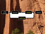
Traffic dynamics with spill-back is solved by systematic relaxation. The systematic relaxation
process performs a multi-agent learning method based on the following sequence:
1. Make an initial guess for the routes of all agents.
2. Execute all agents’ routes simultaneously in a traffic flow simulation (network loading).
3. Re-calculate some or all of the routes using the knowledge of the network loading.
4. Go back to 2.
From the viewpoint of conceptual layers explained above, the route generation happens at
the strategic layer and the network loading (item 2) corresponds to the physical layer. The
queue model considered in this thesis corresponds to the network loading part. It is the model
on which the traffic flow simulation described in this thesis is based.
This thesis is organized as follows: A multi-agent traffic flow simulator, based on the queue
model, for the physical layer of a transportation planning system, called MATSIM [50], is given
in Chapter 2. Chapter 2 also explains the input data, namely the street network and the plans
of travelers, and explains the output data, which is composed of events occurred during the
network loading process. The computational aspects of the sequential execution of the traffic
flow simulator are discussed in Chapter 3. How parallel computing is introduced to the traffic
flow simulation is explained in Chapter 4. Chapter 5 discusses different methods to couple
the strategic and the physical layers of MATSIM. Chapter 6 and Chapter 7 explain how the
different types of data between modules can be exchanged. In particular, how the output data
(events data) is extracted out of the traffic flow simulation and how the input data (plans data)
is got into the traffic flow simulation, respectively. Chapter 8 gives a vision of how the traffic
flow simulation can be used for the Internet packet traffic, and is followed by a summary.
4

Chapter 2
The Queue Model for Traffic Dynamics
2.1 Introduction
A traffic flow simulation consistent with the multi-agent approach discussed in Chapter 1 and
e.g., by [67, 65] should fulfill the following conditions:
The model should have individual travelers/vehicles 1 in order to be consistent with all
agent-oriented learning approaches.
The model should be simple in order to be comparable with static assignment and in
order to allow concentration on computational issues rather than modeling issues.
This includes the ability of task parallelization into software.
The model should be computationally fast so that scenarios of a meaningful size can be
run within acceptable periods of time.
For the work presented here, a fourth condition is also stated:
The model should be somewhat realistic so that meaningful comparisons to real-world
results can be made.
These conditions make the use of existing software packages, such as DynaMIT [17],
DYNASMART [18], or TRANSIMS [59], difficult since these software packages are already
fairly complex and complicated. An alternative is to select a simple model for large scale microscopic
network simulations, and to re-implement it. If one wants queue spill-back, there are
essentially two starting points: queueing theory, and the theory of kinematic waves.
In queueing theory, one can build networks of queues and servers [76, 14, 73]. Packets
enter the network at an arbitrary queue. Once in a queue, they wait typically in a first-in firstout
(FIFO) queue until they are served; servers serve queues with a given rate. Once the packet
is served, it will enters the next queue.
This can be directly applied to car/vehicle traffic, where packets correspond to vehicles,
queues correspond to links, and serving rates correspond to link capacities. The decision of a
vehicle about which link to enter after it is served at an intersection is given by the vehicle’s
route, which is a list of nodes (intersections) that a vehicle must pass through during its trip.
1 Terminology: In multi-agent simulations, agents are units. The traffic flow simulation described here simulates
the vehicle traffic. The agents in the traffic model are vehicles. Agents and vehicles are used on reciprocal
terms. Although a vehicle is an agent of transmission and is generally not restricted to a “car”, it represents a car
and accordingly a driver who is of person-type throughout this thesis.
5

Handling Constraints - Original algorithm
for all links do
while vehicle has arrived at end of link
AND vehicle can be moved according to capacity
AND there is space on destination link do
move vehicle to next link
end while
end for
Figure 2.1: The Gawron’s queue model
A shortcoming of this type of approach is that it does not model spill-back. If queues have
size restrictions, then packets exceeding that restriction are typically dropped [76]. Since this
is not realistic for traffic, an alternative is to refuse further acceptance of vehicles once the
queue is full (“physical queues”). This means that the serving rate of the upstream server is
influenced by a full queue downstream. Gawron presents an example of such a model in [26].
A detailed algorithmic description is given in Figure 2.1.
An important issue with physical queues is that the intersection logic needs to be adapted.
Since without physical queues (i.e. with “point queues”) the outgoing links can always accept
all incoming vehicles, so the maximum flow through each incoming link is just given by each
link’s capacity. However, when outgoing links have limited space, then that space needs to be
distributed among the incoming links which compete for it.
In the original algorithm (Figure 2.1), links are processed in an arbitrary but fixed sequence.
This has the consequence that the most favored link in a given intersection is the one that is
processed next after the congested outgoing link has been processed. This could for example
mean that a small side road obtains priority over a large main road.
A better way to handle this problem is to allocate flow under congested conditions according
to capacity [16]. For example, if there are two incoming links with capacities 2 and 4 vehicles
per time step, and the outgoing link has 3 spaces available, then 1 space should be allocated
to the first incoming link and 2 to the second. Section 2.2.2 explains intersection handling in
more detail.
A shortcoming of queue models is that the speed of the backwards traveling kinematic wave
(“jam wave”) is not correctly modeled. A vehicle that leaves the link at the downstream end
immediately opens up a new space at the upstream end into which a new vehicle can enter,
meaning that the kinematic wave speed is roughly one link per time step, rather than a realistic
velocity. This becomes visible in the dissolution of jams, say at the end of a rush hour: If a
queue extends over a sequence of links, then the jam should dissolve from the downstream end.
In the queue model, it will essentially dissolve from the upstream end. More details of this,
including schematic fundamental diagrams, can be found in [74, 26].
2.2 Queue Model
2.2.1 Gawron’s Queue Model
The so-called queue model introduced by Gawron [26] is used as the base of the traffic dynamics
of the traffic flow simulation. Gawron’s queue model defines three key concepts, namely,
free flow travel time, storage constraint and capacity constraint.
Each link has, from the input files, the attributes free flow velocity ¢¡ , length £ , capacity
6

£
and ¡£¢¥¤§¦©¨ number of lanes . Free flow travel time ¡ ¡ is calculated by . Each vehicle
must spend at least free flow travel time on a link before leaving it.
The storage constraint of a link is defined as the maximum number of vehicles that
£
a
!
link
can hold at the same time. It ¨ ¡¢¤¦¨
is calculated as , where is the space a single
vehicle in the average occupies in a jam, which is the inverse of #"%$'& the jam density. m is
taken throughout this work.
The capacity constraint (flow capacity) of a link, on the other hand, defines an upper-bound
for the number of vehicles that can be released from a link at a given time. This constraint is
given as input.
The intersection logic by Gawron is that all links are processed in an arbitrary but fixed
sequence, and a vehicle is moved to the next link if (1) it has arrived at the end of the link, (2)
it can be moved according to capacity, and (3) there is space on the destination link. Figure 2.1
gives the algorithm. The three conditions mean the following:
A vehicle that enters ( link at ) ¡ time cannot leave the link before ) ¡+*, ¡ time , ¡ where
is the free speed link travel time as explained above.
The condition “vehicle can be moved according to capacity” is determined as
.- or /01 and 23¡£45-7698
where is the integer part of the capacity of the link (in vehicles per time 6 step),
is the fractional part of the capacity of the link, and is the number of the vehicles
which already left the link in the current time 23¡£4 step. is a random number such
¢;:
that
: ¡
. According to this formula, vehicles can leave the link if the leaving
2¦A@ size , i.e. the first integer number being larger or equal than the link capacity (in
vehicles per time step). Vehicles are then moved from the link (the spatial queue) into the
buffer according to the capacity constraint and only if there is space in the buffer; once in
the buffer, vehicles can be moved across intersections without looking at the flow capacity
constraints. This approach is borrowed from lattice gas automata, where particle movements
are also separated into a “propagate” and a “scatter” step [24]. Vehicles move through the nodes
7

node
spatial queue
buffer
acc to capacity
constraint
acc to storage
constraint
Figure 2.2: Simplifying the intersection logic by introducing a separate buffer for each link
besides the spatial queue.
without any delay at the nodes as all the constraints that define eligible vehicles of a link are
determined by the link properties.
As a desired side effect, this makes the update in the algorithm completely parallel: If a
vehicle is moved out of a full link, the new empty space will only open in the buffer and not
on the link, and will thus not become available at the upstream end until the next time step –
at which time it will be shared between the incoming links according to the method described
above. This has the advantage that all information which is necessary for the computation of a
time step is available locally at each intersection before a time step starts – and in consequence
there is no information exchange between intersections during the computation of a time step.
Further details are given in algorithmic form in Figure 2.3.
In order to systematically test the intersection logic, an intersection test suite was implemented
[7]. This test suite goes through several different intersection layouts and tests them
one by one to see if the dynamics behaves according to the specifications. The results of possible
layouts typically look as shown in Figure 2.4.
The curves in Figure 2.4 show time versus the number of vehicles that have left the link so
far. Thus, the slope of the curve equals the measured flow capacity in vehicles per second. For
the data in the figure, one link with a capacity of 500 vehicles/sec and one link with a capacity
of 2000 vehicles/sec merge into a link with a capacity of 500 vehicles/sec. The curves are, for
different algorithms explained below, time-dependent accumulated vehicle counts for the two
incoming links. For approximately the first 50-100 time steps, both incoming links operate at
full capacity (500 and 2000 vehicles/second) and fill the outgoing link. Until approximately
time step 3400, both links discharge at rates 400 and 100 vehicles/sec, respectively. After that
time, the first link is empty, and the second link now discharges at 500 vehicles/sec. Not all
algorithms are similarly faithful in generating the desired dynamics; the thick black lines denote
results from the algorithm which is the current implementation in the traffic flow simulator.
Further details are explained in [7].
In Figure 2.4, Algorithm-1 uses Gawron’s original algorithm as described in Section 2.2.1
and in [26]. This algorithm may lead to wrong results. For example, when a vehicle leaves
a full link, a free space becomes available immediately, so that another vehicle can enter the
link in the same time step. Hence, the results of the simulation are dependent on the sequence
in which the links are processed. As stated above, parallel update is used to get rid of this
problem in the traffic flow simulation.
Algorithm-2 uses the “fair intersections and parallel update” approach described above, and
is provided in Figure 2.3. Algorithm-3, given in Figure 2.5, is very similar to Algorithm-2 ex-
8

Vehicle Movement through Intersections
// Propagate vehicles along links:
for all links do
while vehicle has arrived at end of link
AND vehicle can be moved according to capacity
AND there is space in the buffer (see Fig 2.2) do
move vehicle from link to buffer
end while
end for
// Move vehicles across intersections:
for all nodes do
while there are still eligible links do
Select an eligible link randomly proportional to capacity
Mark link as non-eligible
while there are vehicles in the buffer of that link do
Check the first vehicle in the buffer of the link
if the destination link has space then
Move vehicle from buffer to destination link
Proceed to the next vehicle in the buffer
else
Break the inner while loop and proceed to the next eligible link
end if
end while
end while
end for
Figure 2.3: Vehicle movement at the intersections. Note that the algorithm separates the flow
capacity from intersection dynamics.
600
500
400
Count
300
200
algorithm 1: link 400
algorithm 1: link 200
algorithm 2: link 400
algorithm 2: link 200
algorithm 3: link 400
100
algorithm 3: link 200
algorithm 4: link 400
algorithm 4: link 200
algorithm 5: link 400
algorithm 5: link 200
0
0 1000 2000 3000 4000 5000 6000 7000 8000
Time
Figure 2.4: Test suite results for the intersection dynamics. The curves show the number of
discharging vehicles from two incoming links as explained in section 2.2.2.
9

Algorithm-3 for Vehicle Movement through Intersections:
Same as Alg. 2.3 till this point
// Move vehicles across intersections:
for all nodes do
while there are still eligible links do
Select an eligible link randomly proportional to capacity
if the destination link has space then
Move one vehicle from buffer to destination link
Mark link as non-eligible and proceed to the next link
else
Proceed to the next link
end if
end while
end for
Figure 2.5: Handling intersections according to the modified version of fair intersections algorithm.
Similar to Algorithm 2.3, except that each link, now, can push only one vehicle at a
time.
Algorithm-4 for Vehicle Movement through Intersections:
for all nodes do
if node visited for the first time then
Choose first incoming link randomly
end if
for i = 1..(the number of incoming links) do
Choose next incoming link via Metropolis sampling
if link buffer is empty then
Mark link as non-eligible
else
Take first vehicle in the buffer
if destination link for vehicle has space then
Move that vehicle from buffer to destination link
else
Mark link as non-eligible
end if
end if
end for
end for
Figure 2.6: Handling intersections according to Metropolis sampling.
cept that instead of serving all the “eligible” vehicles from an incoming link to their destination
links, only one vehicle is moved at a time. Hence, Algorithm-3 and Algorithm-2 do not show
any difference when links do not have capacities greater than 1.
Algorithm-4 implements the fair intersections approach with a difference. Selection is done
via Metropolis sampling [55] with one exception: When a node is processed for the first time,
the first incoming link is selected randomly. In general, if the next link has a lower capacity
then the current link ¡ , then the link is selected with a probability that depends on the ratio
of the capacity of link to the capacity of link ¡ . Pseudo code of the algorithm is given in
Figure 2.6.
10

Algorithm 5 for Vehicle Movement through Intersections:
for all nodes do
if node visited for the first time then
Choose first incoming link randomly according to capacity
end if
for i = 1..(the number of incoming links) do
Choose next incoming link via Metropolis sampling
if link buffer is empty then
Mark link as non-eligible
else
Take first vehicle in the buffer
if destination link for vehicle has space then
Move that vehicle from buffer to destination link
else
Mark link as non-eligible
end if
end if
end for
end for
Figure 2.7: Handling intersections according to the modified Metropolis sampling.
Finally, Algorithm-5 is similar to Algorithm-4 except that if a node is visited for the first
time, the first incoming link is selected according to the flow capacity. The algorithm is given
in Figure 2.7.
The queue model reads flow capacities, free speeds and link lengths, from the input files
and accordingly calculates free flow link travel times. The free flow link travel time defines
the minimum time that vehicles on that particular link must spend. Whilst the lower-bound is
known, the upper-bound for a vehicle being on a link before moving to the next link depends on
how long the vehicle waits at the end of the link. If the randomized selection is not in favor of
a link on which a vehicle is ready to move to the next link (Figure 2.3), the travel time related
to the link increases.
There is a remark to be made about flow capacities. When several of very short links (such
as links with a buffer size 1) exist, they reduce the number of vehicles discharge from the longer
links as the available space is reduced by the short links 2 .
2.2.3 Graph Data as Input for Queue Simulation
The traffic flow simulation is fed by the graph data (the street network) and the plans of vehicles
to be executed. Plans are explained in Section 2.2.4. Before the execution of plans, the
simulation reads nodes and links of the street network. The street network is defined in the
XML [97] format and a rough example is shown in Figure 2.8. XML is explained in detail in
2 The problem can be seen as follows: Assume a short link with a given non-integer capacity (per second), with
long links of the same capacity both upstream and downstream. Then, according to standard queuing theory, the
queue length on the short link follows a random walk. However, when that random walk makes the short link
completely full, then the upstream link is no longer allowed to discharge into the short link. Since this happens
fairly often with short links, this means that short links reduce the effective capacity. Note that the effective
capacity reduction is felt for the upstream link. This phenomenon has little effect with the long links of the Swiss
street network defined in Section 2.5, but became apparent with validation studies with the Navtec network of the
Zurich area, which has many short links.
11

- network
- nodes
-
-
-
node i d =”1” x=”651700” y=”137200”/
node i d =”2” x=”652220” y=”137600”/
/ nodes
l i n k i d =”2” from=”2” t o =”1” l e n g t h =”657”
-
c a p a c i t y =”12000” f r e e s p e e d = ”11.1” p e r m l a n e s =”1” /
l i n k i d =”3” from=”1” t o =”2” l e n g t h =”657”
-
c a p a c i t y =”12000” f r e e s p e e d = ”11.1” p e r m l a n e s =”1” /
/ l i n k s -
- l i n k s
- / network
Figure 2.8: An example of the graph data in the XML format
Section 3.4.1.
Each node is identified by a unique ID and x-y coordinates. Each link has the attributes ID,
node IDs that it connects, length, capacity, free flow speed and number of permanent lanes. The
capacity is given in terms of “vehicles per time unit” and refers to the capacity (flow) constraint
of the link.
The graph data example in Figure 2.8 is composed of 2 nodes and 2 links. Links connect
nodes by defining a direction, for example, link 2 is from node 2 to node 1.
Each node in the traffic flow simulation keeps track of its outgoing and incoming links.
When a link of the graph data is read, pointers to it are placed in the arrays for incoming or
outgoing links at the nodes that the link connects. The arrays for outgoing and incoming links
are used, especially, when the movement of vehicles across nodes (intersections) is realized as
written in Figure 2.3. Nodes check the buffers of incoming links for vehicles ready to move to
any of the outgoing links. Furthermore, in the parallel implementation explained in Chapter 4,
the vehicles that move across the boundaries are packed into messages by the nodes.
Each link is mainly composed of a spatial queue and a buffer to separate the flow constraint
from the intersection logic as described earlier. Both the buffer and the spatial queue are nothing
but queues of pointers to vehicles. Besides these two structures, there are 3 more supplementary
queues defined for each link:
Parking queue: holds vehicles of initial legs (see Section 2.2.4) with start times in the
future.
Waiting queue: holds vehicles of initial legs (see Section 2.2.4) whose start time is up
but which cannot make it into the traffic because of full links.
Storage: holds the second or higher legs of vehicles. These legs can be executed only if
the execution of previous legs are completed.
Links are also responsible for putting constraints into practice. Hence, nodes are careless
in terms of constraints. As shown in Figure 2.8, the capacity constraint, which determines the
size of the buffer, is read from the input data. The storage constraint is calculated by using the
length and the number of permanent lanes given in the input data (Section 2.2.1).
2.2.4 Vehicle Plans as Input for Queue Simulation
Vehicles are inserted into one of the queues defined on links (Section 2.2.3) according to their
start times and leg numbers. Hence, the simulation needs to know about the graph data before
12

p e r s o n i d =”6357250”
-
p l a n -
a c t t y p e =”h” x100=”387345” y100=”276590” l i n k =”14584” /
-
l e g mode=” car ” d e p t i m e = ”06:54:35” t r a v t i m e = ”00:30”
-
r o u t e 4 9 0 2 4 9 0 3 4 9 0 4 4 9 0 5 4 9 0 6 4 9 0 7 4 9 0 8 4 9 0 9 - / r o u t e
-
/ l e g -
a c t t y p e =”w” x100=”387345” y100=”276590”
-
l i n k =”14606” dur=”08:00” /
/ p l a n -
- / p e r s o n
Figure 2.9: An example for the plans data in the XML format
reading any vehicle information.
An example of a person’s plan is given in Figure 2.9. Each person has a unique ID and a
plan. A plan is composed of a set of activities. Each activity defines a location, the coordinates
of the location and a link ID, on which the activity will start. Each pair of consecutive activities
describes a leg of the plan. The leg provides information about the means of transportation,
the earliest time that a vehicle can start its execution, the expected travel time from the start
activity location to the end activity location of the leg, and a set of node IDs that defines a route
that is supposed to be followed when moving from the start activity location to the end activity
location.
The traffic flow simulation creates a new agent/vehicle for each leg defined in a person’s
plan. In case a person has more than one leg, the simulation makes sure that the highernumbered
legs wait for the completion of the execution of the previous legs.
2.2.5 Events as Output of Queue Simulation
Since the queue simulation does not aggregate data (Chapter 5.2.1), it only produces events as
the output for the other modules in the system, which are better able to check the correctness
of their own data aggregation. An event is produced whenever a vehicle moves from one queue
to another or leaves the simulation due to various reasons. Possible events are of the following
types (not limited to those listed here):
departure: moving from the parking queue of a link to the waiting queue of the same
link, since the start time has arrived.
leaving a waiting queue: moving from the waiting queue of a link to its spatial queue to
start simulating.
leaving a link: leaving the current link.
entering a link: entering the next link (vehicle leaves the current link just before this
event happens).
being stuck and leaving the simulation: getting stuck in congestion for a specific time
period and leaving the simulation afterwards.
arrival: arrival at the final destination.
A set of events of a vehicle in the XML (Section 3.4.1) format is shown in Figure 2.10.
The example shows the events created while the plan of vehicle 6465 is executed. The vehicle
13

)
¥
§
¡
£
)
¥
)
¥
)
¡
£
)
)
¥
§
*
¡
)
£
¥
)
¥
)
£
)
¥
)
£
e v e n t time = ”06:00” t y p e =” departure ” v e h i d =”6465”
-
legnum=”0” l i n k =”1523” from=”3827”/
e v e n t time = ”06:00” t y p e =” w a i t 2 l i n k ” v e h i d =”6465”
-
legnum=”0” l i n k =”1523” from=”3827”/
e v e n t time = ”06:01” t y p e =” l e f t l i n k ” v e h i d =”6465”
-
legnum=”0” l i n k =”1523” from=”3827”/
e v e n t time = ”06:01” t y p e =” entered l i n k ” v e h i d =”6465”
-
legnum=”0” l i n k =”1524” from=”3828”/
e v e n t time = ”06:28” t y p e =” l e f t l i n k ” v e h i d =”6465”
-
legnum=”0” l i n k =”1524” from=”3828”/
e v e n t time = ”06:28” t y p e =” entered l i n k ” v e h i d =”6465”
-
legnum=”0” l i n k =”1525” from=”3829”/
e v e n t time = ”06:34” t y p e =” a r r i v a l ” v e h i d =”6465”
-
legnum=”0” l i n k =”1525” from=”3829”/
Figure 2.10: An example for the events data in the XML format
starts simulating at 6 AM on link 1523 and during its trip to destination link 1525, it traverses
through link 1524. All the events belong to leg 0. The upstream ends of links 1523, 1524 and
1525 are located at nodes 3827, 3828 and 3829, respectively.
2.3 Other Work
Two arguments against the queue model are often that the intersection behavior is “unfair”
in standard implementations, and that the speed of the backwards traveling jam (“kinematic”)
wave is incorrectly modeled. The first problem was overcome by a better modeling of the
intersection logic, as described in Section 2.2.2. The second problem still remains. What can
be done about it
If one wants to avoid a detailed traffic flow simulation, such as is implemented in TRAN-
SIMS [82] for example, then a possible solution is to use what is sometimes called “mesoscopic
models” or “smoothed particle hydrodynamics” [28]. The idea is to have individual particles
in the simulation, but have them moved by aggregate equations of motion. These equations of
motion should be selected so that in the fluid-dynamical limit the Lighthill-Whitham-Richards
[48] equation is recovered [15].
The number of vehicles in a segment is updated according to
¢¡¤£
¡¦¥
¢¡¤£
©¡
¥
¢¡
¢¡¤£
¥ £
(2.1)
)*
;
*¨§
*
¢¡¤£
©¡
) §
from
¡
segment ¡ ¢¡¤£
) ¡
¢¡¤£
§
where is the number of vehicles in segment at time , is the flow of vehicles
into segment at time , and is the source/sink term given by entry
and exit rates.
What is missing is the specification of the flow rates . A possible specification is
given by the cell transmission model [15]:
¢¡
¢¡ ¡ £
¥ £
¢¡¤£
¥$¥ £
(2.2)
! ¤#"
§% ¤&"('
where §! ¤&" is the capacity constraint, is the jam wave speed, ) is the free speed, * ¤&" is
the maximum number of vehicles on the link and all other variables have the same meaning as
before.
14

)
¥
£
)
¥
©¡%
Note that this now exactly enforces the storage §
constraint by setting
¢¡¤£
to zero
once ¤#" has reached . In addition, the kinematic jam wave speed is given
explicitly
via . There is some interaction between length of a segment, time step, and that needs to
be considered. The network version of the cell transmission model [16] also specifies how
to implement fair intersections. The cell transmission model is implemented under the name
NETCELL [9].
Other link dynamics are, for example, provided by DynaMIT [19], DYNASMART [20] or
DYNEMO [61]. These are based on the same mass conservation equation as Equation
©¡
(2.1), but
¥
use §
different specifications for . In fact, DynaMIT and DYNASMART calculate vehicle
speeds at the time of entry into the segment depending on the number of vehicles already in
the segment. The number of vehicles that can potentially leave a link in a given time step is, in
consequence, given indirectly via this speed computation. Since this is not enough to enforce
physical queues, physical queuing restrictions are added to this description. DYNEMO varies
a vehicle’s speed continuously along the link based on traffic conditions of the current and the
next segment.
2.4 The Basic Benchmark
A real-world scenario is preferred for the benchmarks throughout this thesis instead of using a
synthetic scenario or using only the theoretical performance predictions.
A theoretical performance prediction gives an idea about what is supposed to be expected.
However, such predictions possibly miss some performance-relevant details that appear only
when the real-world data is used. For example, if an example data set is small enough that it
can fit into a computer’s memory while the real-world data is bigger than the available memory,
the results of theoretical predictions for the small data set will include the cache effects. For
example, if the data set can be kept smaller than the size of the cache, which is a high speed
memory system, there might be a significant speed-up since the data is reached with a higher
speed.
Synthetic scenarios are generated by synthetic data. They are used to make generalizations
about the performance of the real-world scenarios. If a real-world scenario with enough information
to test all the features of a benchmark is not available, a synthetic scenario with full
information is useful. Furthermore, the results are easier to adapt between different scenarios
if it is applicable. On the other hand, if a “possible” real-world data needs to cover a lot of
details, then the generation of a similar synthetic scenario gets harder.
2.5 A Practical Scenario for the Benchmarks
One of the conditions that a traffic flow simulation must fulfill is that the simulation should
be able to run scenarios of a meaningful size within acceptable periods of time. From the
transportation planning point of view, such scenarios are large scale real-world problems, which
include millions of agents and all kinds of traffic.
The street network of Switzerland used in the benchmarks of this thesis was originally
developed for the Federal Office for Spatial Development (ARE) [6]. Then, the network was
extended to include the major European transit corridors for a railway-related study [85]. The
version of the street network used through this thesis is a derivation of the extended network.
It contains 10 564 nodes and 28 622 links.
The nodes of the street network are the intersections of roads and are defined by geographical
coordinates. The links are the roads that connect two nodes. Each link is unidirectional and
15

has the attributes such as type, length, speed, and capacity (capacity constraint).
A scenario called ch6-9 is used in the benchmarks through this work. It contains around
1 million trips which start between 6:00AM and 9:00AM. Thus, the scenario used is aimed to
simulate morning rush hour traffic. These trips are based on a realistic demand [65].
The steps followed when converting trips to agents and plans are: (1) a unique agent is
assigned to each trip, and (2) the starting and ending links of a trip become the home and work
locations of the agent. Corresponding activities are created at these locations, so that (3) each
trip becomes a leg between these two activities, and (4) each trip is completed with a route from
the start link to the end link based on free flow travel times in the network.
As stated in Chapter 1, a systematic relaxation is used to carry the initial state of a system to
a relaxed state. With respect to relaxation, the initial plans are fed into the traffic flow simulator
that represents the physical world of the framework as explained in Chapter 1. The results of
the traffic flow simulation are used to improve plans of some agents, which are merged with the
rest of the agents (whose plans have not been changed). The merged plans, then, are fed into
the traffic flow simulator. Each iteration, therefore, involves reading the input files (plans and
graph data), executing all the plans and improving some of the plans according to the output
of the traffic flow simulation. The process is repeated until the system is relaxed, which takes
about 50 iterations. Earlier investigations have shown that this is more than enough to reach
relaxation [68].
During the performance tests of the traffic flow simulation given in the next chapters, the
ch6-9 scenario is simulated for 3 hours, i.e. 10800 time steps (1 time-step means 1 simulated
second).
2.6 Summary
Using a traffic flow simulator for transportation planning is a method for network loading,
which is one of two components in Dynamic Traffic Assignment (DTA). Different criteria such
as resolution (individual vs. aggregated entities), how realistic the behaviors of entities are, the
modes of entities and time resolution determine different traffic flow simulations.
The existent traffic flow simulators are realistic and detailed enough but their complexity
makes them difficult to use. The queue simulation presented here is not only favored in simplicity
but also realistic enough to forecast in future transportation planning [65].
The standard queue-based implementation comes with two main shortcomings: it exhibits
an unfair behavior at the intersections and incorrectly models the speed of backwards traveling
jam waves. The former is remedied by improving the standard intersection behavior as explained
in Section 2.2.2. The solution to the latter is still absent: in the queue model, the traffic
jam dissolves from the upstream end as opposed to that dissolves from the downstream end
in the kinematic wave theory. Some other transportation planning software packages resolve
the problem; however, they either suffer from being too complicated such as the CA model,
or are not modeled at the level of individual entities; in consequence, they lack agent-oriented
approaches.
Despite this remaining shortcoming, the queue model meets the criteria of being comparable
to static traffic assignment, as shown in [65], computing fast, and being receptive to
agent-oriented approaches.
16

Chapter 3
Sequential Queue Model
3.1 Introduction
The queue model is explained in Chapter 2. The computational concern is mentioned as one of
the reasons why the queue model was chosen:
“The model should be computationally fast so that scenarios of a meaningful size
can be run within acceptable periods of time.”
In order to run meaningful scenario sizes, parallel computing is used for the traffic flow
simulation. This will be explained in Chapter 4 in detail. With parallel computing, the same
simulation runs on different computers on different pieces of data. For example, the same
traffic flow simulation code simulates different geographical areas. Because of the parallel
execution, the results can be obtained faster than it can be done with single-CPU execution.
Although parallel programming speeds up the execution of a program, it is not enough by
itself. Improving the single-CPU version of the same program is significant as well in terms of
performance.
The first traffic flow simulator as a part of this thesis was written in C. That simulator
displayed considerable computational performance, but turned out to be difficult to maintain.
For that reason, an alternative traffic flow simulator in C++ [80, 70] was programmed, taking
the advantage of the new possibilities that the Standard Template Library (STL, Section 3.3.1)
offers. However, that new C++ code turned out to be about a factor of two slower than the old
C code.
Many system designers prefer object-oriented programming (such as C++ and Java [42])
because the complexity of systems has increased over the last decades. C++ has become a
dominant programming language for those complex systems. Moreover, recommendations on
how to approach certain problems in C++ have been developed (e.g. [53]). Today, with careful
programming, C++ using the STL can be as fast as C.
For that reason, it was attempted to bring the C++ traffic flow simulator to the same computational
speed as the C traffic flow simulator. This was done by implementing and testing
several different approaches recommended by [53], and by inserting C code into time-critical
pieces of the code. The reason for doing this is to find out where the C++ implementation has
performance disadvantages compared to the C implementation, and how severe these disadvantages
are. Results of the investigation can then be used to make informed decisions regarding
the trade-off between maintainability and computational performance of the code.
17

3.2 The Benchmark
The traffic flow simulator described in Chapter 2.2 is a part of the transportation planning
system explained in Chapter 1. One of the goals of such a system is running a realistic and
meaningful size scenario to make data analysis and predictions. This planning system is not
complete in the sense of common transportation planning, which also includes all modes of
transportation, freight traffic, etc. Such a complete system involves about 7.5 million travelers,
and more than 26 million trips including short pedestrian trips, etc [2].
However, in order to make the transportation planning system explained in Chapter 1 useful
in the real world, a scenario “ch6-9” described in Section 2.5 is used. ch6-9 is a subset of the
data for the full 24-hour car-only simulation, and contains about 1 million trips.
When the traffic flow simulation is coupled with the strategy generation modules via files
as explained in Section 5.2.1, it takes the data from the input files and produces the data into
the output files. The computational performance of the traffic flow simulation is measured
excluding the performance of input reading and output writing. There are two reasons for this:
As investigated in Chapter 6 and Chapter 7, external modules can be defined to handle
input and output of a traffic flow simulation. Using files is just an implementation issue.
Hence, the performance of the simulation itself (i.e., how the graph data and vehicles are
represented, how the data is accessed, how the rules are executed) is the main concern.
I/O requires accesses to the disk where the files are stored. However, I/O performance
is limited by disk speeds, and file I/O operations usually deliver a low performance.
Moreover, using files is just an implementation issue; as explained in Chapter 6 and
Chapter 7, for example, a message passing approach may be used to replace files with
messages.
During the measurements of the traffic flow simulation performance, a 3-hour time period is
simulated. Time steps are incremented by 1 simulation-time second; therefore, the total number
of time steps simulated is 10800. In each time step, 3 basic movements are accomplished:
movement through intersections, movement along links and movement from waiting queues
(where vehicles wait to enter the simulation) to the spatial queues. Each of these movement
steps loops over all the nodes or all the links of the graph data. Accordingly, they dominate the
overall performance.
The figures in the next sections, which show computational performance curves, are plotted
on a multiple-CPU basis since results of some approaches depend on the number of CPUs.
3.3 Performance Issues for C++/STL and C Functions
C++ has been made more functional by the introduction of the Standard Template Library
(STL). The STL is an extensive library of common containers and functions written using C++
templates. In this section, some remarks regarding the experiences with using different STL
containers for different purposes in the traffic flow simulation are given. Although some of the
results just confirm the common sense, some others are specific to the situation that exists in
this work.
The next section gives a brief definition of STL library. The sections following Section 3.3.1
discuss different implementation alternatives and their performance for the different parts of the
traffic flow simulator. Section 3.3.2 compares STL-map and STL-vector used to represent
the street network. Using STL-multimap for the parking and waiting queues of the links in
18

the street network is explained in Section 3.3.3. The same section promotes an alternative data
structure, namely, a self-implemented singly linked list, and gives the test results for these two
implementations. Section 3.3.4 discusses different implementations for the link queues, i.e.,
the spatial queue and the link buffer. The alternatives are using STL-deque, STL-list and
a self-implemented data structure Ring.
3.3.1 The Standard Template Library
The Standard Template Library (STL) is a C++ library composed of the following components:
Collections of standard container types. Containers are implemented as templates, a
special feature of C++ and contain objects of any type. Examples are map, deque
(double-ended queue), vector, list, etc.
Algorithms defined on containers. Examples are: accessing an element, sorting the elements
in a container, searching for an element, etc.
Iterators used for traversing the elements of a container.
The STL not only hides the implementation details of its components but also provides
elegant data structures and algorithms for users. Encapsulation and abstraction properties of
STL enables programmers to focus on application specific issues.
The STL provides two types of containers: Sequence containers store data in a linear sequence.
The “sequence” depends on time and position of insertion. The position of an element
in the container is independent of the element’s value. vector, deque and list are of this
type.
Associative containers, on the other hand, are sorted data structures. They associate the
domain of one type (key) with the domain of another type (value). The position of an element
in such a container depends on its key. Examples are map, multimap, set, etc.
Operations defined on containers, such as insert, delete, or retrieve, differ in performance.
Container selection is dependent on characteristics of the applications and on call frequency.
Some examples are given in next sub-sections.
Each iterator represents a certain position in a container. Regardless of the container for
which it is defined, an iterator comes with a set of basic operators. The basic operators are ++
(stepping forward to the next element), == (equal), != (not equal), = (assignment operator)
and * (dereference operator). Since an iterator is an object, the user must create instances of
the iterator class prior to using them.
3.3.2 Containers: Map vs Vector for Graph Data
Accessing the graph data, i.e. the street network, is one of the key issues in the simulation.
This is because every single item (a link or a node) of the graph is visited several times in each
time step during the simulation run. Moreover, the searching algorithm for the elements of a
container, which represents the graph data, is crucial since searching for a single element in the
graph data is done more than once: (1) when plans are read, the start and the end locations have
to be searched in the graph data, and (2) every time a vehicle on a link at the border needs to
enter the next link, the next link is searched in the graph data to find out, to which computing
node it belongs in the parallel implementation.
The overall approach of using STL containers for the graph data looks as Figure 3.1 (using
graph nodes as the example 1 .)
1 For non-C-experts: typedef aa bb means that from now on, bb will be translated to aa before the
19

make ‘ ‘ Nodes ’ ’ a c o n t a i n e r t y p e :
t y p e d e f CONTAINER- Node Nodes ;
/ / make ‘ ‘ N o d e s I t e r a t o r ’ ’ an i t e r a t o r over Nodes:
t y p e d e f N o d e s : : I t e r a t o r N o d e s I t e r a t o r ;
/ / d e c l a r e the c o n t a i n e r t h a t w i l l c o n t a i n the nodes:
Nodes nodes ;
Figure 3.1: STL-containers for the graph data
The iterator is useful in order to be able to go through all nodes and do something with them
without having to worry about the efficiency of retrieval. Specific examples are given below.
Several operations are, then, needed with respect to that container:
Adding new nodes during initialization.
Going through all nodes in each time step of the simulation (using the iterator).
Finding nodes by their “name” (“key”).
Two implementations were tested: (1) using a map container and (2) using a vector
container.
Map
map is an associative container that can be indexed by any type. Indices (keys) can be simple
types such as integers or sophisticated objects. An STL-map represents a mapping from one
type (key type) to another type (value type). Hence, it allows the management of key-value
pairs.
An advantage of using the STL-map for nodes and links is that it is possible to straightforwardly
retrieve them by their label number: a command such as nodes[1234] is possible
and will retrieve the node with the label number 1234. ID numbers are typically non-sequential,
so it is not possible to use standard array indexing instead.
Sample code using an STL-map for nodes (links are analogous) looks as in Figure 3.2. The
code means that there is a class Node defined somewhere else, and the STL-map container
is loaded with pointers to node instances.
The advantage of using the STL-map is that nodes can be addressed using their IDs using
exactly with the same syntax as one is used from arrays. A slight disadvantage may be the
make pair syntax that one needs to get used to, and the retrieval via second in the iterative
loop. The iterator loop syntax is awkward but standard for all containers.
Vector
An STL-vector is a sequence type of container, which is composed of contiguous blocks of
objects. Element insertion in an STL-vector container can be done at any point in the sequence.
If the insert(position,object) method is used, insertion becomes expensive
at the beginning or in the middle. Since elements are arranged contiguously, all elements that
follow the insertion point need to be shifted. An example of this case is illustrated in Figure 3.3.
compiler does anything else. The statement is particularly useful to convert fairly technical expressions such as
map into something readable such as Nodes (indicating a container that contains nodes).
20

¡
t y p e d e f map- Id , Node Nodes ;
t y p e d e f N o d e s : : i t e r a t o r N o d e s I t e r a t o r ;
Nodes nodes ;
[ . . . ]
r e a d a node i n f o r m a t i o n ;
n o d e s . i n s e r t ( m a k e p a i r ( nodeId , node ) ) ;
[ . . . ]
/ / go through a l l nodes and do something with them:
f o r ( N o d e s I t e r a t o r i t = n o d e s . b e g i n ( ) ;
i t != n o d e s . e n d ( ) ; + + i t )
Node node = i t second ;
node doSomethingWithIt ( ) ;
[ . . . ]
/ / f i n d a node by I d :
Node node = nodes [ t h e I d ] ;
Figure 3.2: The STL-map for the graph data
0 1
2 3 4 5 6
O13 O2 O48 O9 O26 O33 O14
BEFORE CALLING INSERT(3,O19)
0 1 2 3 4 5 6 7
O13 O2 O48 O19 O9 O26 O33 O14
AFTER CALLING INSERT(3,O19)
Figure 3.3: Insertion in the middle of an STL-vector. insert(position,object) is
a method defined on the STL-vector. The elements behind the insertion position are shifted
when insert command is used.
In general, the performance of the insertion into any container depends on the type of container
and where the insertion takes place. In particular, insertion at the end of an STL-vector is
very fast.
Some code elements to use an STL-vector for nodes (once more, links are analogous)
look as in Figure 3.4. The insert of the map is replaced by a push back, which means that
the new node pointer is just added at the end of the STL-vector. The iterator is essentially
the same as before, except that one does not need the second because the element that is
retrieved by it is no longer a (pointer to a) pair, but a (pointer to a) node.
An issue with an STL-vector data structure is now searching for a key, for example to
find the pointer to a node that is denoted by an ID number. A naive solution would be a linear
search, the rough code is shown in Figure 3.5.
21

¡
¥
¥
t y p e d e f v e c t o r- Node Nodes ;
t y p e d e f N o d e s : : i t e r a t o r N o d e s I t e r a t o r ;
Nodes nodes ;
[ . . . ]
r e a d a node ;
n o d e s . p u s h b a c k ( node ) ;
[ . . . ]
/ / s o r t the nodes:
n o d e s . s o r t ( ) ;
[ . . . ]
/ / go through a l l nodes and do something with them:
f o r ( N o d e s I t e r a t o r i t = n o d e s . b e g i n ( ) ;
i t != n o d e s . e n d ( ) ; + + i t )
Node node = i t ;
node doSomethingWithIt ( ) ;
¡
[ . . . ]
/ / f i n d a node by I d :
Node node = findNodeById ( t h e I d ) ;
Figure 3.4: The STL-vector for the graph data
Node findNodeById ( Id t h e I d )
f o r ( N o d e s I t e r a t o r i t = n o d e s . b e g i n ( ) ;
i t != n o d e s . e n d ( ) ; + + i t )
Node node = i t ;
i f ( n o d e . g e t I d ( ) = = t h e I d )
return node ;
¡
¡
/ / node with given Id not found:
e r r o r ( ) ;
Figure 3.5: Linear search for the graph data
However, a better approach is to pre-sort the STL-vector according to the node IDs
and then to use a binary search instead, in which average case and worst case access times
are reduced from
¢¡¤£¦¥
to . Fortunately, both sorting and binary search are already
provided by the STL, so that these are easy to use. The only issue is to provide the sorting
criterion to the algorithm. The code for sorting the elements of the graph data stored in an
STL-vector and the sorting criterion are given in Figure 3.6.
Often, links and nodes are already provided in the correct order by the files. In that case,
initialization time can be further reduced by checking that they are indeed provided in the
22

¡
/ / c a l l i n g s o r t i n g algorithm
void s o r t ( )
s o r t ( n o d e s . b e g i n ( ) , n o d e s . e n d ( ) , c o m p a r i s o n C l a s s ( ) ¡
)
/ / d e f i n i n g comparison c l a s s
c l a s s c o m p a r i s o n C l a s s
p r i v a t e :
/ / comparison f u n c t i o n d e f i n e s ascending order
bool keyLess ( c o n s t i n t & k1 , c o n s t i n t & k2 ) c o n s t
return ( - k1 k2 ) ¡
;
p u b l i c :
/ / comparison based on IDs
/ / comparing two o b j e c t s l h s and rhs
template c l a s s T -
bool operator ( ) ( c o n s t T l h s , c o n s t T r h s ) c o n s t
return keyLess ( ( ( T ) l h s) i d ( ) , ( ( T ) r h s ) i d ( ) ) ;
¡
/ / comparing an o b j e c t l h s with a value k
- template c l a s s T
bool operator ( ) ( c o n s t T l h s , c o n s t i n t & k ) c o n s t
return keyLess ( ( ( T ) l h s) i d ( ) , k ) ;
¡
;
/ / comparing a value k with an o b j e c t rhs
- template c l a s s T
bool operator ( ) ( c o n s t i n t & k , c o n s t T r h s ) c o n s t
return keyLess ( k , ( ( T ) r h s ) i d ( ) ) ;
¡
Figure 3.6: Sorting the graph data stored in an STL-vector
correct sequence, and thus sorting can be skipped.
Results
Figure 3.7 shows the simulation runtime results for using the STL-vector and the STL-map
structures representing graph data. Figure 3.7(a) plots the data points for RTR. RTR means Real
Time Ratio, which shows how much faster simulation runs than real life. Figure 3.7(b) contains
the speed-up, which shows how much the execution speeds up by increasing the number of
traffic flow simulators running in parallel in the system. The concepts of RTR and speed-up are
covered in detail in Chapter 4. The data points are labeled as “Single” and ”Double”, which
means that the results are gathered by running either single simulation or two simulations per
computer, respectively.
Performance gain using the STL-vector for the graph data instead of the STL-map is
seen in Figure 3.7. In these tests, the STL-multimap (Section 3.3.3) is used as the data
structure for the parking queues and waiting queues and the self-implemented Ring structure
23

1024
RTR, Diff. Data Str. for Graph Data
256
Speedup, Diff. Data Str. for Graph Data
512
256
64
Real Time Ratio
128
64
32
16
8
Single, Vector
4
Single, Map
Double, Vector
Double, Map
2
1 2 4 8 16 32 64 128
Number of CPUs
Speedup
16
4
1
0.25
1 2 4 8 16 32 64 128
Number of CPUs
Single, Vector
Single, Map
Double, Vector
Double, Map
(a)
(b)
Figure 3.7: RTR and Speedup for using different data structures for the graph data. “Single”
means only one traffic flow simulation is run per computing node. “Double” refers to running
two traffic flow simulations per computing node. In this test, an STL-multimap is used for
parking and waiting queues, the Ring class is used for spatial queues and link buffers.
(Section 3.3.4) represents the spatial queues and buffers of the links.
Using the STL--vector relatively accelerates the traffic flow simulation by 15% for the
large number of CPUs and for the small number of CPUs the relative performance increase
observed is up to 18% compared to results of the STL-map. The STL-map performance
mainly suffers from searching and accessing an item in the container. Hence, the STL-map
can be replaced by the STL-vector and the search algorithm can be changed to the binary
search for better performance.
Map vs Vector for Graph Data: Recommendations
Although using the STL-vector to represent the graph data elements, namely nodes
and links, along with the STL’s binary search algorithm is 15-18% faster than using
the STL-map and the STL-map’s find method, it comes with higher programming
overhead. For the cases that require faster computation, the STL-vector is recommended.
If one prefers to skip the programming overhead, the STL-map should be
chosen.
3.3.3 Containers: Multimap vs Linked List for Parking and Waiting
Queues
Parking and waiting queues are zones where a vehicle waits until it is ready to start to simulate.
In other words, a vehicle waits in these containers until its start time for the simulation is up.
A person’s plan can have more than one leg. Each leg is defined as a route between two
locations. If a person has a plan, which includes a trip from home to work and then from work
to leisure, then it means the person’s plan has two legs.
When a person’s plan is read by the simulation, a vehicle is created for each leg. If it is the
first leg, then the vehicle is added to the parking queue of the link at which the vehicle starts. In
each time step, the parking queue of each link is checked for vehicles that are ready to start at
the current time step. Those vehicles are moved to the waiting queue of the link. If the spatial
24

t y p e d e f multimap- Time , Veh WaitQueue ;
WaitQueue waitQueue ;
t y p e d e f multimap- Time , Veh ParkQueue ;
ParkQueue parkQueue ;
Figure 3.8: Declarations for waiting and parking queues with the STL-multimap
t y p e d e f Linked- Time , Veh WaitQueue ;
WaitQueue waitQueue ;
t y p e d e f Linked- Time , Veh ParkQueue ;
ParkQueue parkQueue ;
Figure 3.9: Declarations for waiting and parking queues with linked lists
queue is not full, the vehicle is moved from the waiting queue into the spatial queue so that it
can start its trip.
Hence, in each time step, waiting and parking queues are checked for the eligible vehicles.
In realistic scenarios, most of the vehicles wait in these queues because their drivers are actually
performing an activity. Checking for all eligible vehicles and accessing their information and
moving them to other queues when necessary comes with computational cost. Therefore, an
appropriate data structure should be used for these queues. That data structure needs to make
available the vehicle with the next scheduled departure at low performance cost. For this, a
partial ordering would in fact be sufficient. However, there is no data structure in the STL
which supplies a fully efficient partial ordering. Therefore, two fully ordered data structures
were tested: the STL-multimap, and a self-implemented singly linked list.
Note that this section only discusses waiting and parking queues. Data structures for link
cells will be explained in the next subsection.
Multimap
An easy-to-use fully sorted data structure is the STL-multimap. One just inserts key-item
pairs, with the keys equal to the start time of vehicles and the items being pointers to vehicles,
and the resulting data structure is automatically sorted. The difference between the STL-map,
as mentioned above, and the STL-multimap is that the latter accepts multiple elements for
the same key. This is necessary since it is possible that several vehicles want to depart at the
same time step. The declarations by using STL-multimap are given in Figure 3.8.
User-defined singly linked list
There are three operations defined on these queues: Insertion of an element into a queue, retrieving
the first element of the queue, and deleting the first element of the queue. Unfortunately
these operations are rather costly with the STL-multimap. From the experiences in the C
version of the simulation where a linked list was been used for these queues, a linked list is
implemented also in the C++ version to handle waiting and parking queues.
The Linked class in Figure 3.9 represents a singly linked list where each item in the list
has a pointer to the next item. Insertion at the end of the list and insertion according to a key
value into the sorted list are available. The latter is important so that vehicles can be sorted
according to their start times.
25

1024
RTR, Diff. Data Str. for Parking and Waiting Queue
256
Speedup, Diff. Data Str. for Parking and Waiting Queue
512
256
64
Real Time Ratio
128
64
32
16
8
Single, Linked List
4
Single, Map
Double, Linked List
Double, Map
2
1 2 4 8 16 32 64 128
Number of CPUs
Speedup
16
4
1
0.25
1 2 4 8 16 32 64 128
Number of CPUs
Single, Linked List
Single, Map
Double, Linked List
Double, Map
(a)
(b)
Figure 3.10: RTR and Speedup for using different data structures for waiting and parking
queues. An STL-vector is used for the graph data and the Ring class is used for the spatial
queues and the link buffers.
Results
Figure 3.10 shows RTR and speed-up results for the simulation runtime on the STL-multimap
and the linked list implementations of waiting and parking queues. In these tests, the vector
container of STL is employed for the graph data (Section 3.3.2), and the spatial queues and
links buffers are implemented by using the self-implemented Ring class (Section 3.3.4.
The linked list implements the queues with a better performance. Quantitatively, the linked
list version increases the performance relatively by 9% as the number of CPUs increases. With
the small number of CPUs, the relative gain is about 18%.
Multimap vs Linked List for Parking and Waiting Queues:Recommendations
Using a singly linked list class with proper methods similar to STL’s containers is recommended
over the STL-multimap since not only the operations on it are faster but
also the implementation details can be hidden from users as done in STL’s containers.
3.3.4 Containers: Ring, Deque and List Implementations of Link Queues
Each link of the traffic flow simulator has two more queues: one for the spatial queue and
one for the buffer used in through-node movement as explained in Chapter 2. In contrast to
Section 3.3.3, the link and the buffer queues are true FIFO (First In First Out) data structures,
and they have finite size.
The way links operate is important in terms of performance since the links are accessed
several times in each time step of the simulation:
The waiting queue of each link is checked to see if there are vehicles to move from the
waiting queue to the spatial queue.
Each spatial queue is checked to see if there are vehicles to move into the buffer of the
link according to the capacity constraint.
The buffer of each link is checked to find out if there is any vehicle to move to the next
link.
26

In this section, two STL functions will be tested, namely, list and deque. Because of the
low performance they involve, in addition a user-defined data structure Ring is implemented
and tested.
List
The STL-list is a doubly linked list. With the STL-list, insertion anywhere is fast but
it provides only sequential access. Since random access is not needed, this should in theory
be a fast data structure for the purpose here. Unfortunately, the STL-list comes with high
overhead as explained below.
Deque
The STL-deque (double-ended queue) is similar in usage and syntax to the STL-vector.
It allows random access and inserts elements fast at either end. Therefore the STL-deque
is the data structure of choice when most insertions and deletions take place at the beginning
or at the end of a container. The STL-deque is different from the STL-vector in terms
of memory management. When resizing is necessary, the STL-deque allocates memory in
chunks as it grows, with room for a fixed number of elements in each reallocation. In other
words, the STL-deque uses a series of smaller blocks of memory. The STL-vector, on the
other hand, allocates its memory in a contiguous block, i.e., the STL-vector is represented
by one long block of memory.
Self-implemented Ring data structure
To overcome the inefficiencies of the STL-list and the STL-deque, a new data structure,
Ring is implemented. Ring is a circular vector. Removal is at the beginning and insertion
is at the end. Removing from the beginning of the STL-vector is a costly operation since
it includes the forward movement of all the remaining elements. In order to get rid of this
difficulty, supplementary pointers are used to keep track of the head and the tail of the data
structure. Hence, with this new structure, only head/tail pointers move back and forth, not the
elements as in the STL-vector container. The same pointers are also used for insertion.
Figure 3.11(a) shows how insertion takes place at the end of Ring structure. The supplementary
pointers head and tail are used to keep track of elements. The maximum size of the
structure is 8 in the example. When the size is 0, the head and the tail point to NIL. Then, an
object, O1, is requested to be inserted. A pointer to the object is placed in the first cell of the
structure. Both the head and the tail point to this cell (accordingly O1) after the insertion. Then
another object, O2, is to be inserted. Since the call is push back, it is placed at the end, i.e.,
the next cell after the last item (O1). The tail pointer is advanced. Now, the head points to O1
and the tail points to O2. The current size becomes 2.
Figure 3.11(b) illustrates deletion from the beginning, by using pop front. The structure
is full, i.e., the size is 8. The head points to the first element(O1) and the tail points the last
element (O8). After deletion, the tail remains the same, but the head is advanced to the next
object (O2) from O1. If further deletion is requested, the head is moved one more cell (to O3).
After two deletions, the size becomes 6.
It is important to note that this works because of the fixed maximum size. This corresponds
to the maximum number of vehicles on the link.
27

push_back(O1)
push_back(02)
head = NIL
head
O1
head
O1
tail = NIL
tail
tail
O2
(a) Insertion at the end
O7
O8
O7
O8
O7
O8
pop_front()
pop_front()
O6
tail
O1
O6
tail
O6
tail
head
head
head
O5
O2
O5
O2
O5
O4
O3
O4
O3
O4
O3
(b) Deletion at the beginning
Figure 3.11: Operations on the Ring structure. (a) Insertion at the end. (b) Deletion from the
beginning.
1024
RTR, Diff. Data Str. for Link Queues
256
Speedup, Diff. Data Str. for Link Queues
512
256
64
Real Time Ratio
128
64
32
16
Single, Ring
8
Single, Deque
Single, List
4
Double, Ring
Double, Deque
Double, List
2
1 2 4 8 16 32 64 128
Number of CPUs
Speedup
16
4
1
0.25
1 2 4 8 16 32 64 128
Number of CPUs
Single, Ring
Single, Deque
Single, List
Double, Ring
Double, Deque
Double, List
(a)
(b)
Figure 3.12: RTR and Speedup for using different data structures for the spatial queues and
the buffers. An STL-multimap is used for parking and waiting queues. An STL-vector is
used for graph data.
Results
Figure 3.12 shows the comparison results for using the STL-list, the STL-deque and the
Ring class as the main data structure of the queues of links. In these tests, the vector
container of STL represent the graph data (Section 3.3.2), and the parking and waiting queues
are handled via the STL-multimap (Section 3.3.3.
The STL-list gives the worst performance. This is because of the memory management
of the STL-list design. A well known example is that to store an integer value (4 bytes),
the STL-list needs 12 bytes plus the list itself. On the other hand, for example, an STLvector
needs only 4 bytes to store an integer. The Ring class speeds up the performance the
best, and the STL-deque performance is between the STL-list and the Ring class.
Changing the data structure from the STL-list to the STL-deque speeds up the execution
relatively by 67% for the large number of traffic flow simulators in the system despite the
28

difference being around 13% with the small number of CPUs. Transition from the STL-list
to the Ring class results in 71% and 29% relatively better performance with the small and the
large number of CPUs, respectively.
Ring, Deque and List for Link Cells:Recommendations
Since users can implement their own containers similar to STL’s containers to overcome
the inefficiencies that appear at the application level, a circular vector called,
Ring, is recommended when the maximum number of elements in a container is
known. When there is no upper limit on the number of elements, the STL-deque is
suggested if most of the insertions and deletions take place at the either ends. When
random access is not required, the STL-list should be chosen.
3.4 Reading Input Files for Traffic Simulators
In applications with different cooperating modules, the format used to represent shared data
becomes more significant. There is no single good solution for this problem since the possible
solutions give either good performance or flexibility but not usually both at the same time. How
the input data is kept in the simulation exhibits the same problem.
This section and the next section investigate the input files (the street network and plans)
and the output file (events) of a traffic simulator, respectively. In this section, comparison of
representing data in the XML [97] format or in the structured text file format is achieved in
terms of I/O performance along with the programming issues with respect to these formats.
The different programming issues tested for plans (Section 3.4.3) are reading XML plans
using expat and reading raw plans from a structured text file using the C++ input operator
and the C function fscanf. Reading the street network information from an XML file using
the expat parser is compared to reading the same information from a structured text file by
using the C function sscanf in Section 3.4.4.
3.4.1 The Extensible Markup Language, XML
XML [97] is the abbreviation for Extensible Markup Language. It is a markup language, which
has the virtues of HTML (Hypertext Markup Language). HTML [11] is widely used especially
for putting data on the World Wide Web such that anyone can access the data without regard
to the location or the time. HTML is known for its simplicity and portability. HTML focuses
on the appearance of documents, not their contents. Hence, it is limited on its features. This
limitation causes XML, which is oriented towards content, to become very popular as a markup
language.
XML is simple, portable, easily maintainable and adaptable. One can design his/her own
customized markup languages by using XML since data is stored in a self-explanatory manner.
For example, the following shows a valid XML tag with 6 valid attribute-value pairs. Each
attribute-value pair is in attribute=”value” format.
l i n k i d =”2” from=”2” t o =”1” l e n g t h =”657” c a p a c i t y =”12000” f r e e s p e e d = ”11.1” /¢
¡
Some of the benefits of using XML files are
XML allows users to create their own sets of tags.
29

The sequence of attributes is not important since when reading data in, the search is done
for the attribute names to obtain the corresponding values. Therefore, new attributes can
be added in any sequence, and rearranging does not cause changes in reading code.
Complex input like trees and hierarchies can be implemented.
XML allows users without prior knowledge to understand the language as it is selfdescribing.
XML promotes flexible context-dependent data, e.g. the description of a bus trip within
a leg can be completely different from the description of a car trip within a leg.
3.4.2 Structured Text
The structured text file format is application-dependent. Therefore, it is user-defined in many
cases. The structured format used here is the column-based format. The example below is the
corresponding column-based text line of the XML example given above. However, without
looking at the XML tag above, it is impossible to understand what these numbers mean. Because
the numbers in a column-based text file are unlikely to be self-explanatory. One might
put a title line at the top of the file to explain what each column corresponds to. It could help
when the number of columns is small like the example below. If each line is composed of, for
example, 30 columns, then it becomes difficult to follow the columns of the lines.
2 2 1 6 5 7 1 2 0 0 0 1 1 . 1
When reading a structured text file, which is composed of a set of numbers, the numbers
need to be read in the same sequence as they are written in the file. Rearranging or inserting
new columns between the columns that are already there requires changes in file-reading code
to keep the consistency with the correct sequence. Despite this drawback, the structured text
files are usually better than the XML format files performance-wise.
3.4.3 XML vs. Structured Text Files: Plans Reading
The plans (Section 2.2.4) contain all the information about agents, including their routes. A
scenario with approximately 1 million agents is kept in a structured text file size of 34 MBytes
and in an XML file size of 330 MBytes. The XML file is 10 times bigger because of the
self-explanatory attributes of XML.
When reading an XML file, the attributes are parsed. An XML parser called expat [21],
which is written in C, is employed. What a parser does is to provide users with opening element
tags (), and the text data.
Afterwards, the users should implement code to handle the values passed in.
In the structured text plans file case, a fixed number of integers is read and according to some
of these numbers another chunk of integers is read to complete a single agent’s information.
A rough example of this type, reflecting the example in the XML format shown in Figure 2.9,
is illustrated below. All the numbers regarding each plan can be written in a single line. The
example separates them into several lines for readability purposes.
6 3 5 7 2 5 0 0 2 4 8 7 5
1 4 5 8 4 1 4 6 0 6 1 8 0 0
0 8
4 9 0 2 4 9 0 3 4 9 0 4 4 9 0 5 4 9 0 6 4 9 0 7 4 9 0 8 4 9 0 9
30

XML File, expat Structured Text File, Structured Text File, fscanf
159s 31s 36s
Table 3.1: Performance results for reading different types of plans file and approaches.
In the example, 6357250 is the vehicle ID, 0 in the first line shows the leg number, and
24875 is the start time of the plan in seconds (06:54:35). The start accessory ID and the end
accessory ID are 14584 and 14606, respectively. An accessory can be an activity location, a
parking or a transit stop. Duration of the leg is 1800 seconds (30 minutes). The 0 in the third
line shows the mode of transport (car). 8 is the number of the intermediate nodes between the
start and the end activity locations, and these nodes are lined up in the last line.
The performance is user-implementation dependent. One version of implementation keeps
each vehicle’s data in integers in an STL-vector while reading. When the vehicle is created,
the program accesses the values from the STL-vector. The code elements are given in
Figure 3.13.
Yet another version uses a C library function called fscanf to read chunks of data. The
data is directly stored into integer arrays similar to the STL-vector used above. Once the
vehicle is created, its variables are set using these integer arrays. A rough example code is
given in Figure 3.14.
Results
Table 3.1 shows the results for different reading approaches and for different types of the plans
file. The scenario used is the one explained in Section 2.5, i.e., around 1 million agents are
read. The numbers show the time for reading and for constructing agents. Once the agents are
created, they are inserted into one of the supplementary structures of the links, such as waiting
queues and parking queues. These queues are of the STL-multimap type.
Reading the same data from the structured text plans file gives better results by 80% relative
to the XML file version. Despite its lower performance values, XML is a promising technology
because of its benefits as given in Section 3.4.1.
An important remark to be made is that the lower performance values of XML come mostly
from the implementation inefficiencies, not from format itself: While expat parses the input
plans file, an object-oriented wrapper around expat inserts each person’s data (plans and the
other attributes) into an STL-deque. If the traffic flow simulator needs to read the next person,
the wrapper calls pop front() to get and to remove the first element from the STL-deque.
A problem resides here: The STL-deque is used in a way that it keeps the objects as opposed
to keeping pointers to the objects. When a pop front() call is made on such a container,
before deleting the element, the wrapper copies the element into a temporary variable. Then,
the element is deleted from the STL-deque and the temporary variable is returned (copied)
to the traffic flow simulator. If one used pointers to objects instead of objects themselves, not
only memory allocation would be done once and in an efficient way but also the pointers to
objects would be copied between different components via copying pointers instead of copying
the objects themselves, which that would result in less overhead.
3.4.4 XML vs Structured Text Files: Graph Data Reading
The graph data can also be kept in two different types of files. Nodes and links are defined by
either XML attributes or column-based numbers. The XML graph data file reading is the same
31

¡
¡
¡
c l a s s Plan
/ / data s t r u c t u r e s
/ / v e c t o r f o r the elements of the f i x e d l e n g t h part
v e c t o r- i n t f i x e d P a r t ;
/ / v e c t o r f o r the elements of the v a r i a b l e l e n g t h part
v e c t o r- i n t v a r i a b l e P a r t ;
d e f i n e s e t and g e t methods t o a c c e s s both v e c t o r s
void r e a d N e x t P l a n ( i f s t r e a m p l a n s f i l e )
/ / read f i x e d l e n g t h p a r t :
f o r ( each item i i n f i x e d l e n g t h p a r t of p l a n )
/ / read an i n t e g e r and put i t i n t o the v e c t o r
p l a n s f i l e f i x e d P a r t [ i ] ;
¡
/ / read v a r i a b l e l e n g t h part ( r o u t e s ) :
/ / number of items in v a r i a b l e l e n g t h part
/ / i s s t o r e d in f i x e d part
f o r ( each item j i n v a r i a b l e l e n g t h p a r t of p l a n )
/ / read an i n t e g e r and put i t i n t o the v e c t o r
p l a n s f i l e v a r i a b l e P a r t [ j ] ¡
;
;
. . . .
main ( )
/ / d e f i n e the plans input f i l e
i f s t r e a m p l a n s f i l e ;
/ / c r e a t e a plan o b j e c t
P l a n s myPlan ;
while ( n o t EOF )
m y P l a n . r e a d N e x t P l a n ( p l a n s f i l e )
c r e a t e a new v e h i c l e
use g e t methods of myPlan t o s e t d a t a of v e h i c l e ¡
s
Figure 3.13: Reading plans from a structured text file, by using an STL-vector
as the XML plans reading: a parser parses the file and the user code saves the values. The size
of the XML graph data file for the network defined in Section 2.5 is around 4 MBytes.
If the same graph data file is a column-based text file, the file size is 2 MBytes. It is read
line by line and each column is extracted from the line. This version uses C library function
sscanf to pick the values after reading each line.
32

¡
¡
main ( )
/ / c r e a t e an i n t e g e r array
/ / f o r the elements of the f i x e d l e n g t h part
i n t f i x e d P a r t [MAXSIZE ] ;
/ / c r e a t e an i n t e g e r array
/ / f o r the elements of the v a r i a b l e l e n g t h part
i n t v a r i a b l e P a r t [MAXSIZE ] ;
while ( n o t EOF )
/ / read f i x e d l e n g t h p a r t :
f o r ( each item i i n f i x e d l e n g t h p a r t of p l a n )
/ / read an i n t e g e r item from f i l e i n t o the array
f s c a n f ( f i l e , i n t e g e r , f i x e d P a r t [ i ] ) ¡
;
/ / read v a r i a b l e l e n g t h p a r t :
f o r ( each item j i n v a r i a b l e l e n g t h p a r t of p l a n )
/ / read an i n t e g e r item from f i l e i n t o the array
f s c a n f ( f i l e , i n t e g e r , v a r i a b l e P a r t [ j ] ) ¡
;
c r e a t e a new v e h i c l e
s e t t h e v e h i c l e v a r i a b l e s using v a l u e s s t o r e d i n a r r a y s
Figure 3.14: Reading plans from a structured text file, by using fscanf
XML File, expat Structured Text File, sscanf
1.14s 0.66s
Table 3.2: Performance results for reading the graph data
Table 3.2 shows that reading graph data of the scenario described in Section 2.5 from a
column-based text file is 1.7 times (relatively 42%) faster than that from an XML file. The
elements of the graph data are stored in an STL-vector.
XML vs Structured Text Files:Recommendations
The choice for the format of a file between structured text files and XML files is a
trade-off between flexibility, extensibility, elegancy and good performance. If the computational
issues can be ignored for an application, using XML files is recommended.
3.5 Writing Events Files
Events generated by traffic flow simulators are fed back to different modules in the framework
as explained in detail in Section 5.2.1. Among the different modules are the router, agent
database, activity generator, etc. When modules in a system are coupled via files, writing files
33

Writing Time
Explanation Raw
Local Disk, C++ 61s
via NFS , C++ 81s
Local Disk, C 57s
via NFS, C 66s
Table 3.3: Performance results for writing the events file.
(plans and events) might also be interesting to investigate. In the framework, plans are written
by the agent database based on the routes generated by the router before the simulation starts.
The performance issues for plans writing are explained in Section 5.2.3.
Events, on the other hand, are written by traffic flow simulators during each simulation
run. In this section, writing raw events using the C++ output operator
and the C function
fprintf is tested on disks that are both local and remote to the machine on which the traffic
simulator runs. The results 2 are shown in Table 3.3.
By default, during the tests reported throughout this thesis, the files and the runtime executables
of MATSIM [50] are all on local disks of the computing nodes. Therefore, no I/O
operations via network are performed unless it is said so. In the table, the label Local Disk
shows no network contribution.
The Network File System (NFS) [72] allows machines to mount a disk partition on a remote
machine as if it was on a local hard disk. NFS comes with a cost because it accesses the remote
files using the network. The cost can be seen in the table. Contribution of NFS in these numbers
shows a performance degradation by a factor of ¡ $¢¡£¡ .
The file writing is accomplished both with C and C++ I/O functions, namely, with the
fprintf function and the operator. The results show that there is a little performance
difference between C and C++ I/O functions when the files are on local disks. When the files
are written via NFS, the difference becomes more apparent.
Another remark is that using endl in output streams of C++ makes the writing into a file
much slower than using \n. Besides adding a newline character as \n does, endl also flushes
the output buffer. Therefore a write() system call is done for each line of operation,
which is an expensive operation. The C++ type writing results in the table are from using \n.
Reading and Writing Big Files:Recommendations
If a big file is read as strings, using C functions such as strtod/strtol and
atoi/atof to convert strings to the appropriate data types should be preferred.
C++ operator can be used to read the data directly into correct types without
any conversion, but this method comes with lower performance. Similarly, the C++
output operator is a bit slower than the C function fprintf. However, when
the performance issues are not taken into consideration, C++ operators and
should be chosen since their usage is very straightforward.
2 The theoretical performance prediction for writing events is investigated in Section 6.8.4
34

3.6 Conclusions and Discussion
Computationally fast programs can be achieved by not only introducing parallel programming
techniques into an implementation, but also accelerating the sequential parts of the implementation.
When a data structure is accessed for its entities frequently, the type of data structure has a
prominent effect on performance. The sequential implementation of the traffic flow simulation
is improved such that:
Storage for graph data is modified in a way that the STL-map is replaced by STLvector
and the searching algorithm is modified to use binary search. The performance
gets better by 15-18% compared to the STL-map version.
Storage for parking and waiting queues, on which vehicles at the beginning, are often
accessed and removed, are advanced from the STL-multimap to a user-implemented
singly linked list structure that results in a 9-18% performance increase.
Representation of link cells as an STL-list degrades performance by 13-67% compared
to using the STL-deque. Even better speed-up (40-71% relative to the STLlist)
is achieved when using a user-defined data structure called Ring, which is nothing
but a circular STL-vector composed of pointers to vehicles.
Operations on files depend on the format of data stored in them. The XML-type files
are flexible in terms of management and are elegant, but they usually give worse performance.
The inherent simplicity of structured text files offer better performance but a lack
of flexibility limits their applicability.
The input stream operator >> of C++ promotes easy usage by letting users to not worry
about types of input to be read, but suffers from low performance.
Therefore, the following conclusions are drawn for the best design of MATSIM:
As the graph data, i.e. the links and nodes, being the most frequently accessed data, it is
best represented by the STL-vector. The binary search algorithm of STL should be
used finding an element in the vector structure.
The parking and waiting queues of the links are the data structures which hold the vehicles.
The vehicles on these queues have not started simulating yet either because of full
links or because of travelers performing activities at the location. Removing all the eligible
vehicles at the beginning of these queues prior to inserting them into other queues,
and inserting new vehicles into these queues are best performed on a data structure defined
as a singly linked list so that each vehicle points to another vehicle.
The spatial queues and buffers of the links are best implemented by using a fixed size
vector, elements of which are pointers to vehicles. The movement operations such as
insertion and deletion should be based on pointers to vehicles.
For the input and output data, XML files should be preferred to structured text files since
XML allows constructing user defined complex structures in a more efficient way.
35

RunTime Graph Data Parking-Waiting Queues Link Queues
615s STL-vector STL-multimap STL-list
533s STL-vector STL-multimap STL-deque
438s STL-vector STL-multimap Ring
539s STL-map STL-multimap Ring
356s STL-vector Linked List Ring
Table 3.4: Summary table of the serial performance results for different data structures of the
traffic flow simulator.
3.7 Summary
The concepts of fast computation and easy-to-use programming methods can be coupled. C has
been around since 1970s and has allowed programming at both higher and lower levels. However
as more complex applications come into prominence, new languages are needed since:
these applications are complicated enough, content-wise; new programming techniques
that ease the burden of programmers for complex applications are preferred, and
these applications usually exhibit a hierarchy of entities.
Object-oriented languages such as C++ [70, 80] and Java [42] are written to fill the deficiencies
of C-type languages and are used to handle the complexity of applications.
The first implementation of the traffic flow simulator was written in C. Despite being computationally
fast, it obstructed adding new features easily. Writing in C++ with the improvements
explained in the previous sections provides a simulation, which not only is computationally
fast, but also has hierarchical entities, which are re-usable and as a matter of fact easy to
use as well as easy to mutate. Naturally, some arguments presented here might be specific to
the implementation achieved.
Table 3.4 summarizes different implementations for the containers in the traffic flow simulator.
The run times shown in the table are from the time measurements when the number of
computing nodes (CPUs) is chosen as 1. The results exclude any file input and output operations
as explained in Section 3.2. The input file reading results are already shown in Table 3.1
and in Table 3.2 for plans and the street network, respectively. The output file writing results
for events are given in Table 3.3.
36

Chapter 4
Parallel Queue Model
4.1 Introduction
Serial computation has been around for years. With this traditional computing manner,
problems run on a single computer/computing node,
instructions of a program are executed one after the other by the CPU,
only one instruction may be executed at a time.
Data transmission through hardware, which is limited by the speed of light [83], determines
the speed of a serial computer. In addition to physical constraints, there are also economic limitations
since it is increasingly expensive to make a single processor faster. These limitations
make it harder to build faster serial computers by saturating the performance of serial computers.
Ultimately, the agent-based simulation of large scale transportation scenarios are concerned.
A typical scenario would be the 24-hour (about seconds) simulation of a metropolitan area
consisting of 10 million travelers. Typical computational speeds of ¡ ¢¡ traffic flow simulations
with 1-second update steps are 100 000 vehicles in real time [58, 56, 68]. This results in a
computation time of ¡ ¢ ¡£¢£¢
¡ ¢ ¢
seconds ¤ days. This number is just a rough
estimate and subject to the following changes: Increases in CPU speed will reduce the number;
¡ ¢ ¡ ¢£¢
more realistic driving logic will increase the number; smaller time steps [64, 84] will increase
the number.
This means that such a traffic flow simulation running on a single computing node is too
slow for practical or academic treatment of large scale problems. In addition, computer time is
needed for activity generation, route generation, learning, etc. In consequence, it makes sense
to explore parallel/distributed computing as an option. Parallel/distributed computing has the
advantages of using non-local resources, competitive cost/performance ratio and overcoming
finite memory constraint of single computers that are subject to. In parallel computing computational
problems are solved by using several computing resources which may consist of a
single computer with multiple processors or a number of computers connected through a network,
which is called a PC cluster, or a combination of both. In order to solve a computational
problem through parallel computing, one must think about (i) how to partition the tasks into
subtasks, and (ii) how to provide the data exchange between the subtasks. Before explaining
these issues, parallel architectures will be discussed in the following paragraphs.
The categorization of parallel computers has been done in many different ways, among
which Flynn’s Classical Taxonomy [83] is the one most commonly used. This classification
37

depends on the dimensions (single or multiple) of instructions and data. Each combination
gives a different category:
Single Instruction Single Data (SISD): Same instruction stream executes one data stream
which causes deterministic execution. Most PCs, single CPU workstations and mainframes
have this feature.
Single Instruction Multiple Data (SIMD): Same instruction stream executes different data
on different computing nodes. Examples are CM-2, IBM 9000, Cray C90.
Multiple Instruction Single Data (MISD): Different instruction streams run on the same
data. It is the one less commonly used.
Multiple Instruction Multiple Data (MIMD): The most popular type of parallel computers.
Each processor runs a different set of instructions on different data. Execution can be
synchronous or asynchronous, deterministic or non-deterministic. Most supercomputers
and PC clusters are of this type.
4.1.1 Message Exchange
This work concentrates on clusters of coupled PCs, i.e., Linux [39] boxes connected through
100 Mbit Ethernet [77] Local Area Network (LAN). Using this type of clusters, which is costeffective,
can achieve a performance close to that of a vector computer [57]. This is, in part, due
to the fact that multi-agent simulations do not vectorize well, so that vector computers offer no
particular advantages. Hence, PC clusters are expected to be the dominant high performance
computing technology in the area of multi-agent traffic flow simulations for many years to
come.
With respect to data exchange between subtasks, there are, in general, two main approaches
to inter-processor communication. One of them is called message passing between processors;
the alternative is called shared-address space, where variables are kept in a common pool
globally available to all processors. Each paradigm has its own advantages and disadvantages.
In the shared-address space approach, all variables are globally accessible by all processors.
Despite multiple processors operating independently, they share the same memory resources.
The shared-address space approach makes it simpler for the user to achieve parallelism but
since the memory bandwidth is limited, severe bottlenecks are inevitable with an increasing
number of processors, or alternatively such shared memory parallel computers become very
expensive. For those reasons, message passing is the focus point.
In the message passing approach, there are independent cooperating processors. Each processor
has a private local memory in order to keep the variables and data, and thus can access
local data very rapidly. If an exchange of the information is needed between the processors,
the processors communicate and synchronize by passing messages, which are simple send and
receive instructions. Message passing can be imagined to be similar to sending a letter. The
following phases happen during a message passing operation.
1. The message needs to be packed i.e. the computer is told which data needs to be sent.
2. The message is sent.
3. The message may then take some time on the network until it finally arrives in the receiver’s
inbox.
4. The receiver has to officially receive the message, i.e. to take it out of the inbox.
38

5. The receiver must unpack the message and tell the computer where to store the received
data.
There are time delays associated with each of these phases. It is important to note that some
of these time delays are incurred even for an empty message (“latency”), whereas others depend
on the size of the message (“bandwidth restriction”). Effects of time delays are explained in
Section 4.4.
4.1.2 Domain Decomposition
On PC clusters, two general strategies are possible for parallelization of data domains:
Task parallelization – The different modules of a transportation simulation package
(traffic flow simulation, routing, activities generation, learning, pre-/postprocessing) are
run on different computers. This approach is for example used by DynaMIT [17] or
DYNASMART [18].
The advantage of this approach is that it is conceptually straightforward, and fairly insensitive
to network bottlenecks. The disadvantage of this approach is that the slowest
module will dominate the computing speed – for example, if the traffic flow simulation
among different modules is using up most of the computing time, then task parallelization
of the modules will not help.
Domain decomposition – In this approach, each module is distributed across several
CPUs. In fact, for most of the modules, this is straightforward since in current practical
implementations activity generation, route generation, and learning are done for each
traveler separately. Only traffic flow simulation has tight interaction between the travelers
as explained in the following.
For PC clusters, the most costly communication operation is the initiation of a message
(“latency”). In consequence, the number of CPUs that need to communicate with each other
should be minimized. This is achieved through a domain decomposition (see Figure 4.2) of the
traffic network graph. As long as the domains remain compact, each CPU will, on average, have
at most six neighbors (Euler’s theorem for planar graphs). Since network graphs are irregular
structures, a method to deal with this irregularity is needed. METIS [91] is a software package
that specifically deals with decomposing graphs for parallel computation and is explained in
more detail in Section 4.3.1.
The quality of the graph decomposition has consequences for parallel efficiency (load balancing):
If one CPU has a lot more work to do than all other CPUs, then all other CPUs are
¡ ¢ ¢
obliged to wait for it, which is inefficient. For the current work with CPUs and networks
¢ ¢ ¢ ¢
with links, the “latency problem” (explained in Section 4.4) always dominates load
balancing issues; however it is generally useful to employ the actual computational load per
network entity for the graph decomposition [57].
For shared memory machines, other forms of parallelization are possible, based on individual
network links or individual travelers. A dispatcher could distribute links for computation
in a round-robin fashion to the CPUs of the shared memory machine [31]; technically, threads
[72] would be used for this. This is be called fine-grained parallelism, as opposed to the coarsegrained
parallelism, which is more appropriate for message passing architectures. As stated
above, the main drawback of this method is that one needs an expensive machine if one wants
to use large numbers of CPUs.
39

4.2 Parallel Computing in Transportation Simulations
Parallel computing has been employed in several transportation simulation projects. One of the
first was PARAMICS [8], which started as a high performance computing project on a Connection
Machine CM-2. In order to fit the specific architecture of that machine, cars/travelers were
not truly objects but particles with a limited amount of internal state information. PARAMICS
was later ported to a CM-5, where it was simultaneously made more object-oriented. In [8], a
computational speed of 120 000 vehicles with an RTR (real time ratio, see Section 4.4) of 3 is
reported, on 32 CPUs of a Cray T3E.
At about the same time, it was shown that on coupled workstation architectures it is possible
to efficiently implement vehicles in object-like fashion, and a parallel computing prototype
with “intelligent” vehicles was developed [56]. This later resulted in the research code PAM-
INA [68], which was the technical basis for the parallel version of TRANSIMS [57]. In the
tests (using Ethernet [77] only, on a network with 20 000 links, about 100 000 vehicles simultaneously
in the simulation), TRANSIMS [57] ran about 10 times faster than real time with
the default parameters, and about 65 times faster than real time after tuning. These numbers
refer to 32 CPUs; adding more CPUs did not yield further improvement. The parallel concepts
behind TRANSIMS are the same as behind the queue model described in Chapter 2, and in consequence
TRANSIMS is up against the same latency problem as the queue model. However,
for unknown reasons the computational speed is lower than predicted by latency alone.
Some other early implementations of parallel traffic flow simulations are discussed in [10,
60]. A parallel implementation of AIMSUN [23] reports a speed-up of 3.5 on 8 CPUS using
threads (which uses the shared memory technology as explained above) [4].
DYNEMO [71] is a macro-particle model, similar to DYNASMART [18] described below.
A parallel version was implemented about five years ago [61]. A speed-up of 15 on 19 CPUs
connected through 100 Mbit Ethernet was reported on a traffic network of Berlin and Brandenburg
with 13738 links. Larger numbers of CPUs were reported to be inefficient.
DynaMIT [17] uses functional decomposition (task parallelization) as a parallelization concept
[17]. This means that different modules, such as the router, the traffic flow (supply) simulation,
the demand estimation, etc., can be run in parallel, but the traffic flow (supply) simulation
runs on a single CPU only. Functional decomposition is outside the scope of this thesis.
DYNASMART [18] also reports the intention of implementing functional decomposition.
Note that in terms of raw simulation speed, the performance values presented in this work
are more than an order of magnitude faster than anything listed above. In addition, this is not
achieved by a smaller scenario size, but by diligent model selection, efficient implementation,
and by hardware improvements based on knowledge where the computational bottlenecks are.
That is, this approach makes it possible to run very large scale scenarios as everyday research
topics, rather than to have them as the result of computationally intensive studies only.
4.3 Implementation
As discussed in the previous sections, the parallel target architecture for this traffic flow simulation
is a PC cluster. The suitable approach for this architecture is domain decomposition, i.e.
to decompose the street network graph into several pieces, and to give each piece to a different
CPU. Information exchange between CPUs is achieved via messages.
When parallelization of a transportation simulation, one needs to decide where to split the
underlying street network, and how to achieve the message exchange. Both questions can only
be answered with respect to a particular traffic model, but lessons learned here can be used for
40

PROC P0
PROC P1
N3
N1
N2
Figure 4.1: Handling the boundaries and split links
other models.
4.3.1 Handling Domain Decomposition
In general, one wants to split as far away from the intersection as possible. This implies that one
should split links in the middle, for example, as TRANSIMS [57] does. However, for the queue
model “middle of the link” does not make sense since there is no real representation of space. In
consequence, one can either split at the downstream end or at the upstream end of the link. The
downstream end is undesirable because vehicles driving towards an intersection are influenced
by the intersection to a greater degree than vehicles driving away from an intersection. For that
reason, in the queue simulation one splits the nodes right after the intersection (Figure 4.1).
A good partitioning algorithm must decompose a domain in such a way that each subpart
gets a fair share of the load. This issue is also known as load balancing. Load balancing
ensures that no single CPU is overloaded or idle. In the application presented throughout this
thesis, a software package called METIS [91] is employed for domain decomposition. It has
been chosen since it gives good results with large irregular graphs, which would describe the
underlying street network given in Section 2.5.
METIS differs from the traditional graph partition algorithms because of multilevel partitioning
algorithms it uses. The traditional graph algorithms do the partitioning directly on the
original graph. They are usually slow and do not result in good quality.
METIS uses multilevel recursive bisection or multilevel k-way partitioning for higher quality
results. Multilevel recursive bisection performs a sequence of bisections on the graph. It
does not necessarily result in the best quality partitioning, however it is widely used because of
its simplicity.
The multilevel k-way partitioning of METIS is utilized throughout this thesis. It is a 3-phase
partitioning technique:
The original graph is coarsened down to fewer nodes by collapsing nodes and links. This
41

350000
300000
250000
200000
150000
100000
50000
450000 500000 550000 600000 650000 700000 750000 800000 850000
Figure 4.2: Decomposed street network of Switzerland extracted from the map of whole Europe,
on which METIS software package is used. The number of partitions is 8 in this example; 7
of them are colored separately; the 8th partition is also colored and shows the rest of Europe,
hence it is cut here.
makes it easier to find the best partition boundary of the graph.
Then, k-way partitioning is achieved on the smaller large-grained graph.
Finally, the decomposed graph is uncoarsened to find a k-way partitioning of the original
graph.
Both multilevel recursive bisection and multilevel k-way partitioning also aim to reduce the
edge-cut, which is the number of split links whose nodes belong to different partitions. A result
of METIS partitioning Switzerland’s street network can be seen in Figure 4.2.
4.3.2 Handling Message Exchanging
Once the domain decomposition method breaks a problem into several subproblems, single
or multiple programs are executed over subproblems on different computing nodes at the same
time. It is common that the subproblems are not fully independent, i.e., exchanging information
at the boundaries of different subproblems is necessary.
With respect to the application presented here, message passing implies that a CPU that
“owns” a split link reports, via a message, the number of empty spaces to the CPU, which
“owns” the intersection from which vehicles can enter the link. After this, the intersection
update can be done in parallel for all intersections. Next, a CPU that “owns” an intersection
reports, via a message, the vehicles that have moved to the CPUs, which “own” the outgoing
links. Pseudo code of how this is implemented using message passing is shown in Figure 4.3.
In fact, the algorithms in Figure 2.3 and Figure 4.3 together give the whole pseudo code for
the parallel queue model traffic dynamics. For efficiency reasons, all messages to the same
CPU in the same time step should be merged into a single message in order to incur the latency
overhead only once.
4.3.3 Communication Software
The communication among the processors can be achieved by using a message passing library,
which provides functions to send and receive data. There are several libraries such as MPI
(Message Passing Interface) [51] or PVM (Parallel Virtual Machine) [63] for this purpose. Both
42

Algorithm – Parallel computing implementation
According to Alg. 2.3, propagate vehicles along links.
for all split links do
SEND the number of empty spaces of the link to the other processor.
end for
for all split links do
RECEIVE the number of empty spaces of the link from the other processor.
end for
According to Alg. 2.3, move vehicles across intersections.
for all split links do
SEND vehicles which just entered a split link to the other processor
end for
for all split links do
RECEIVE the vehicles (if any) from the neighbor at the other end of the link.
place these vehicles into the local queues.
end for
Figure 4.3: Parallel implementation of queue model.
PVM and MPI are software packages/libraries that allow heterogeneous PCs interconnected by
a computer network to exchange data. They both define an interface for different programming
languages such as C/C++ or Fortran. For the purposes of parallel traffic flow simulation, the
differences between PVM and MPI are negligible. In principle, CORBA (Common Object
Request Broker Architecture) [92] would be an alternative to MPI or PVM, in particular for
task parallelization; but practical experiences show that it is difficult to use and because of the
strict client-server paradigm is not well suited to the systems, which assume that all tasks are
on equal hierarchical levels.
Among these approaches, MPI is chosen since it has slightly more focus on computational
performance. Some key features of MPI can be summarized as follows:
The specification of MPI is machine independent, i.e., data exchange among different
machine architectures will not cause any data loss because of different word lengths of
the machines. This is also a feature of PVM.
Different processes of a parallel program can execute different executable binary files
(i.e. task parallelization). This is also provided by PVM.
MPI does not dictate specific behavior on errors other than indicating what the error is.
This is because MPI expects users to go with high-quality implementations knowing that
determined error recovery specifications will limit the portability of MPI.
MPI allows processes to be defined in different inter-communicators. Different intercommunicators
are capable of communicating with each other. As explained in Chapter
7, this helps coupling different modules available in the application presented here.
MPI is designed to operate on different communication technologies. MPI is used both over
Ethernet [77] and Myrinet [54]. Moreover, PVM is tested on the same technologies, however,
the results for PVM on Myrinet do not outperform results for PVM on Ethernet. Here a brief
definition of Myrinet technologies is given. The results and comparison figures can be found
in Section 4.5.
43

¢¡ ¥
¡
* 6
§¡ ¥
¢¡ ¥
8
£
Myrinet [54] is a high-performance packet-communication and switching technology designed
by a company called Myricom to provide a high-speed communication medium for PC
clusters. Compared to other technologies, Myrinet has much less protocol overhead than others,
and therefore provides much better throughput and latency. One-way latency of Myrinet
is 6 secs [54]. 10Gbit Ethernet reportedly has an end-to-end latency of 21 secs [36]. A
measurement using ping command on the Fast Ethernet LAN reports a round-trip latency of
0.20-0.25 msecs.
PCs in a cluster interconnected by Myrinet are linked via low-overhead routers and switches
as opposed to connecting one machine directly to another. Most of the fault-tolerant features
such as flow control, error control etc., are backed up by the low-overhead switches.
4.4 Theoretical Performance Expectations
The problem size and the memory requirement of a sequential program are the determining
factors of measuring the performance of the program. If the memory need of a sequential
program can be supplied by the system, the execution time of the program becomes directly
proportional to the problem size. Thus, prediction of the performance of a sequential program
is straight-forward.
As far as parallel programs are concerned, the problem size and the memory are still the
essential factors but they are not enough to explain the more complicated behavior of parallel
programs. When measuring the performance of a parallel program, load balancing and communication
overhead complicate the determination of parallel performance measurement.
Performance of parallel programs can be monitored by different metrics. Among these
metrics, execution time and speed-up are the most commonly used. In addition to these two
metrics, another metric called real-time ratio is concerned. RTR describes how much faster
than reality the simulation is running.
In a log-log plot, the speed-up curve can be obtained from the RTR curve by a simple
vertical shift; this vertical shift corresponds to a division by the RTR of the single-CPU version
of the simulation. Speed-up curves put more emphasis on the efficiency of the implementation
and less emphasis on absolute speed. An additional difference is that speed-up is independent
of the problem size except at the Ethernet saturation level, which depends on the problem size,
while RTR depends on problem size except for the Ethernet saturation level, which does NOT
depend on the problem size.
The execution time of a parallel program is defined as the total time elapsed from the time
the first processor starts execution to the time the last processor completes the execution. During
execution, on a PC cluster, each processor is either computing or communicating. Consequently,
¥ §¡ £
¦¥ ¨£¢
¦£¢
¦¥ ©£©
¢¡ ¥
¦¥ £©
where is the execution time, is the number of processors, is the computation time and
is the communication time.
For a problem that can be parallelized using domain decomposition, the time required for
the computation, , can be approximated in terms of the runtime of the computation on a
single CPU divided by the number of processors. also includes the overhead effects
such as handling the boundary conditions by both CPUs and unequal domain size effects, i.e.,
load balancing problems. Therefore, the theoretical value can be written as
¢¡ ¥
7¤£© ¦¥
¢¡ ¥
* ¤£©
(4.1)
¤¥ ¦£©
/ ¡
(4.2)
¡¦¥
¤£© ¦¥
44
* 6 ¦

¡
¡
¤
¤
¦
£
¤
¦
£
£
where 6 and 6# ¦ are the overhead and load balancing effects, ¨£© ¦¥
¡¦¥
is the serial execution
¡
6 6 ¦
¤£© ¤¥
time 1 and is the number of CPUs. Under the circumstances of and being small
enough, is approximated as:
§¡ ¥
¤¥ ¦£©
¤£© ¦¥
¡¦¥
(4.3)
¡
Communication ¤£¢ time, , generally has two contributors: bandwidth and latency.
Bandwidth is the transfer rate of data, for example measured in terms of bytes per second.
It is defined by at least two contributions: node bandwidth, and network bandwidth. Node
bandwidth is the bandwidth of the connection from a CPU to the network. If two computers
communicate with each other, this is the maximum bandwidth they can reach. Hence, this is
sometimes also called the “point-to-point” bandwidth.
The node bandwidth contribution to the communication time is expressed as
§¡ ¥
(4.4)
¥A¢
where ¥ ¢
¢¡ ¥
is the number of split links in the ¥A¢
simulation;
the message size.
§¡ ¥ ¡
is the number of split
links per computational and¡
node is
The network bandwidth is given by the technology and the topology of the network. Typical
technologies are 100 Mbit Fast Ethernet, Gigabit Ethernet, etc ([77]). Typical topologies are
bus topologies, switched topologies, two-dimensional topologies (e.g. grid/torus), hypercube
topologies, etc. For example, a traditional Local Area Network (LAN) uses 100 Mbit Ethernet,
with a shared bus topology. In a shared bus topology, the same medium is used for all
£¢
communications between computers, i.e, they have to share the network bandwidth.
In a switched topology, the network bandwidth is given by the backplane of the switch.
Often, the backplane bandwidth is high enough to have all nodes communicate with each other
at full node bandwidth, and for practical purposes one can thus neglect the network bandwidth
effect for switched networks.
Communication time involves the network bandwidth formulated as:
£¢
¢¡ ¥¡
(4.5)
¥ ¢
The cluster used for the tests through this work has a switched topology. Thus,¤
¦©¨ comes
from the technical data of the central switch.
Latency, the second contributor of communication time, is the time necessary to initiate the
communication. Latency is the limiting factor of 10/100 Mbit Ethernet LANs. New technologies
such as Gigabit Ethernet and Myrinet promote lower latencies.
If all the contributing factors are taken into account, the communication time per time step
is formulated as follows:
¤
¦¨
¥¢
¢¡ ¥
¥¦¨§
¥
¡
¡
¥A¢
(4.6)
/ ¡ ¦©§
§¡
¥ ¢
¡
¦¨
8 ¤
¦£©
9¢> *¨
which will be explained in the following paragraphs.
is the number of sub-time-steps. Since two boundary exchanges per time step are
done, for the application represented in this thesis.
£¦§ ¥¦¨§
1 The serial or sequential execution time of a problem can be measured by running the problem on a single
computing node.
45

¥¦¨§
¡¦©§
§¡ ¥
*
§¡ ¥
¡
/ ¡
¢¡ ¥
¡
¢
¡
¡
¡ *
¡
¡
¥
¡
¡ ¡¦¥ £ ¡ ¡¦¥
£
¡
* 6
¡
¡
*
¡
¡
¢¡ ¥
¡
¡
£ ¡ *
*
¡
£
$
£
§¡ ¥
¡
£
¤
¦©¨
$ (4.10)
¢
¡
¡ ¢
¡
£ ¡ ¡¦¥
£ ¡ ¥
¤
¡ ¥
¡¦§is the number of neighbor domains each CPU communicates to. All information, which
goes to the same CPU, is collected and sent as a single message, thus incurring the latency only
once per neighbor domain. For , ¡9¦©§is zero since there is no other domain to communicate
with. For , it is one. For and assuming that domains are always connected, Euler’s
theorem for planar graphs says that the average number of neighbors cannot be more than six.
Figure 4.4 shows an area composed of hexagons. Each hexagon represents a computing
node and the total number of computing nodes is . Thus, the figure shows the domain decomposition
of the area on partitions. The hexagons are painted with 4 different colors. Each
color represents a different number of edges of hexagons shared with the neighbors. The spectrum
has four colors in the figure, namely, the conditions for 2,3,4 and 6 neighbor-cases are
handled from lightest to darkest in this order. The total number of edges shared by neighboring
partitions is calculated as follows: Two of the hexagons (1st and th) have 2 neighbors; two of
the hexagons ( th and th) have 3 neighbors; of the hexagons (the
remaining ones on the edges) have 4 neighbors and of the hexagons (the ones in the
middle) have 6 neighbors. Thus, the average number of neighbors becomes:
¥
¤ *¦¥ *
£ ¡ ¥
*¦¥
£ ¡ ¥
(4.7)
¡ ¦©§
§¡
The numerator of the formula is an integer if
argument in Equation 4.7, the following is used
¡
and is even. Based on the geometric
(4.8)
which has ¡9¦©§
¡¦¥
formula, ¡¦§
¡ ¡ ¢
¥ as desired, and for .
is the latency (or start-up time) of each ¡ ¢> message. as said above, is between 9¢> 0.20-0.25
milliseconds for the Fast Ethernet network of the cluster used throughout this thesis.
Consequently, the combined time for one time step is
¡¦§
¢¡ ¥
§¡ ¥
¢¡ ¥
§¡ ¥
8 * (4.9)
* 6 ¦
¥ ¢
¥¢
£¢
¢¥ *¨§ (
¥A¢
i.e., ¡¦§
According to the discussion above, for ¡ ¡ ¢
the number of neighbors becomes constant,
¤
¦
£ ¡
and the number of split links in the simulation converges to £ ¡
¡©)
. In consequence, 6 for 6 ¦ and small enough:
©
, i.e., ¥ ¢
for a shared or bus topology,¤
¦¨ is relatively small and constant, thus
£ ¡ ¡ £ ¡
for a switched or a parallel supercomputer topology, one assumes¤
¦¨+
and obtains
¡ ¡
¡ *
£ ¡
Thus, in a shared topology, adding CPUs will eventually increase the simulation time, thus
making the simulation slower. In a non-shared topology, adding CPUs will eventually not
make the simulation any faster, but at least it will not be detrimental to computational speed.
46

¢
1
P 1/2 elements
P 1/2
1/2
(P −2)elements
1/2
(P −2)elements
P
Figure 4.4: Calculation of neighbors of computing nodes
¡ ¢
The dominant term in a shared topology for is the network bandwidth; the dominant
term in a non-shared topology is ¡ the latency.
By taking the latency of 100 Mbit Fast Ethernet cards as 0.225 ms, the following calculation
is done to find out the saturation level of Fast Ethernet. Each processor sends messages twice
¡
per time step to all neighbors resulting in latency $'" § contributions or per time step.
In other words, the cluster can maximally do ¢ $'" ¡ " time steps per second. If the time
step of a simulation is one second, then with a 100 Mbit Ethernet, 370 is also the maximum real
¡ ¢ ¢
time ratio of the parallel simulation, i.e. the number which says how much faster than reality
the simulation is. Note that the limiting value does not depend on the problem size or on the
speed of the algorithm; it is a limiting number for any parallel computation of a 2-dimensional
system on a PC cluster using Ethernet LAN.
The only way this number can be improved under the assumptions made is to use faster
communication hardware. Gigabit Ethernet hardware is faster, but standard driver implementations
give away that advantage [45]. In contrast, Myrinet [54] is a communication technology
specifically designed for this situation. Interestingly, as will be seen later, it is possible to
recoup the cost for a Myrinet network by being able to work with a smaller cluster.
47

4.5 Experimental Results
The parallel queue model is used as the traffic flow simulation within the project of a microscopic
and activity-based simulation of all of Switzerland. Computational performance results
are reported here; validation results with respect to a real world scenario can be found in [65].
The cluster used during the tests is composed of 32 computers each of which is a Pentium
III 1GHz dual CPU node. Besides a default 10 Mbit Ethernet [77] communication layer between
these computing nodes, two more network interfaces were available: Fast Ethernet [77]
and Myrinet [54]. Throughout the rest of this thesis, the term Ethernet will refer to Fast Ethernet.
Fast Ethernet is the follow up of 10 Mbit Ethernet technology. It offers a speed of 100 Mbit/s.
Even though it is 10 times faster than 10 Mbit Ethernet, they are both specified by the same
standards. Due to further developments in the Ethernet technology, Gigabit Ethernet giving a
data rate of 1Gbit/s has also come into the picture.
In terms of software, all computing nodes are dual boot: RedHat Linux [40] and Microsoft
Windows [13]. However, all the tests achieved in this work are done only on Linux. More
information about the cluster technology used throughout this work is given in [46].
The following performance numbers refer to the scenario “ch6-9” explained in Section 2.5
containing around 1 million agents and a street network with 10 564 nodes and 28 622 links.
Moreover, as also stated in Section 2.5, the scenario is simulated for 3 hours excluding input
reading and output writing.
In the following sections, different computing issues are discussed: Section 4.5.1 compares
the execution times of the parallel traffic flow simulation over different communication media,
namely, Ethernet and Myrinet. The communication libraries, PVM and MPI are tested and
the results are shown in Section 4.5.2. Packing the number of empty spaces on the links of
the street network and packing the vehicles moving across the boundaries by using different
packing algorithms are discussed in Section 4.5.3. Finally, employing different options of
METIS decomposition library is given in Section 4.5.4.
4.5.1 Comparison of Different Communication Hardware: Ethernet vs.
Myrinet
The most important plot is Figure 4.5(a). It shows computational real time ratio (RTR) numbers
as a function of the number of CPUs. Note that, with 60 CPUs with Myrinet, an RTR of 900
is achieved. This means that 24 hours of all car traffic in Switzerland are simulated in less
than two minutes! This performance is achieved with Myrinet communication hardware; by
using 100 Mbit Ethernet hardware, peak performance is at about 300 RTR. Due to the lack
of availability of more computing nodes, the tests could not go further than 60 in terms of
number of computing nodes. But the practical results follow the predicted curve for RTR for
the available computing nodes.
When the measurement is taken for the curves in Figure 4.5(a), the spatial queues and
buffers of the links implemented by the self-implemented Ring class as explained in Section
3.3.4. The graph data is stored in an STL-vector (Section 3.3.2). Finally, the supplementary
data structures such as waiting and parking queues are implemented by using the
linked list structure described in Section 3.3.3.
The plot also shows two different graphs for achieving the performance with single-CPU
or with dual-CPU machines; obviously there are differences, which are less important. The
lower values of dual-CPU machines are due to the fact that the bandwidth of the network
card is shared between two processes running on a single machine. However, the performance
48

1024
RTR for a 3-hour run of 6-9 Scenario
256
Speedup for a 3-hour run of 6-9 Scenario
512
128
256
64
Real Time Ratio
128
64
32
16
8
single,myri
single,eth
4
double, myri
double, eth
Theo. Val
2
1 2 4 8 16 32 64 128 256
Number of CPUs
(a)
Speedup
32
16
8
4
2
Single, Myri
1
Single, Eth
Double, Myri
Double, Eth
0.5
1 2 4 8 16 32 64 128 256
Number of CPUs
(b)
Figure 4.5: RTR and Speedup curves for Parallel Queue Model. The results are measured when
spatial queues and link buffers are of the Ring type, waiting and parking queues are Linked
List and the graph data is stored in an STL-vector. See Chapter 3 for further details.
decrease of dual-CPU machines compared to single-CPU machines is less than a factor of
1.5, which is presumably due to the fact that one process can communicate while the other is
computing.
One advantage of dual-CPU machines is encountered when investigating the cost/performance
ratio. The cost of a single-CPU machine is only a little lower than that of a dual-CPU machine.
Furthermore, the performance difference between these two setups, as stated above, is less than
a factor of 1.5. For example, RTR for using 56 computing nodes on Fast Ethernet is 300 and
284 with single-CPU and dual-CPU machines, respectively. The cost of 56 single-CPU machines
is around twice the cost of 28 dual-CPU machines. Thus, the cost/performance ratio of
dual-CPU machines is competitive to that of single-CPU machines.
There is a super-linear speed-up between 32 and 60 computing nodes when Myrinet is used.
This is presumably due to cache effects, i.e., the sub-domains become small enough that their
data fits into cache.
The theoretical curve for execution time in Figure 4.5(a) is calculated as follows. The computation
time, , is taken from Equation 4.3 where is the measurement taken from a
¤£¢
¥ ¢¡
¦¥
sequential run executing one time step. The measured value is about 0.065. The communication
time is ¤£© formulated as
§¡ ¥
¥
where, as stated earlier, £¦§equals to 2, ¡9¦§
¢¡ ¥
is calculated from Equation 4.8. Finally, ) ¢¤ is
the latency measured at 0.225 milliseconds on the cluster.
In Figure 4.5(b), the corresponding speed-up curves are shown. As stated in Section 4.4,
speed-up curves can be obtained by shifting RTR curves vertically. The shifting factor is about
5 here. A speed-up of 32 with 60 CPUs is reached when using Myrinet.
The most important results can be summarized as follows:
¤£©
)¢¥¤§
§¡ ¥
; ¥¦§
¡¦©§
§¡
On PC clusters (Linux boxes) with Ethernet, parallel traffic flow simulation speed
theoretically saturates at 370 simulation time steps per second. With the maximum
nodes that can be used, the practical values show the commitment to the theoretical
curve. This statement is independent of scenario size or size of the PC cluster. —
In contrast, on PC clusters with Myrinet, no saturation effect was observed for the
scenario sizes considered.
49

¡
¥
¡
If the simulation time step is one second, then “300 simulation time steps per second” translates
into a real time ratio of 300, meaning the simulation runs 300 times faster than real time.
It is interesting to compare two different hardware configurations:
56 single CPU machines using 100 Mbit LAN.
Real time ratio 300.
¢¡
¥
Cost approx &
switch, ¡
resulting in ¡
¢¡
¡ ¡ ¢¡
for the machines plus approx for a full bandwidth
overall.
¢£¡
28 dual CPU machines using Myrinet.
Real time ratio 900.
Cost approx ¥¤
¡
, Myrinet included.
¤ $&
That is, the Myrinet setup is not only faster, but somewhat unexpectedly also cheaper. A
Myrinet setup has the additional advantage that smaller scenarios than the one discussed here
will run even faster, whereas on the Ethernet cluster, smaller scenarios will run with the same
computational speed as large scenarios.
As mentioned in Section 4.4, the speed-up curves show the same performance saturation as
do the RTR curves. Even larger scenarios reach greater speed-up, but saturate at the same RTR
on Ethernet.
Improving the single version of the simulation explained in Chapter 3 also appears in parallel
computing results. For example, Figure 3.7 shows the results when improving the data
structure used for the graph data.
4.5.2 Comparison of Different Communication Software: MPI vs. PVM
During tests, MPI [51] is used as communication software. Yet, PVM [63] is also utilized to
see whether it makes a difference. One might say that software performance is limited with
hardware performance. However, it is also significant how software is designed to get the most
benefit from hardware.
PVM and MPI have been compared for years. For the purposes of the application presented
here, their capabilities are rather similar as explained in Section 4.3.3. Figure 4.6 compares
the results of using PVM or MPI. The curves are created when an STL-map is used for the
graph data (Section 3.3.2), when the parking and waiting queues are represented by an STLmultimap
(Section 3.3.3, and when the Ring class, as explained in Section 3.3.4 is employed
for the spatial queues and link buffers.
When the underlying computer network is chosen to be Ethernet, MPI and PVM perform
similarly. Presumably, for Ethernet being commonly used as a communication infrastructure
imposes on software developers to improve software designed based on it. When a special
infrastructure, such as Myrinet, is used, the support it gets is proportional to the demand by
the users. Both MPI and PVM support Myrinet but personal experiences show that only MPI
is able to exploit the hardware advantage of Myrinet: As seen in Figure 4.6, PVM on Myrinet
behaves as if it runs on Ethernet. The reasons for this remain unclear; the attempts of developers
of PVM over Myrinet for instrumenting the software on the cluster could not reach a solution.
The important consequence is:
If one wants to use high performance communications hardware, such as Myrinet or
Infiniband, for PC clusters, then the use of MPI is strongly recommended since it is
significantly better supported than any other parallel communication standard.
50

1024
512
256
RTR for a 3-hour run of 6-9 Scenario, PVM TEST
256
128
64
Eth-MPI
Myri-MPI
Eth-PVM
Myri-PVM
Speedup for a 3-hour run of 6-9 Scenario, PVM TEST
Real Time Ratio
128
64
32
16
Speed-Up
32
16
8
4
8
Eth-MPI
4
Myri-MPI
Eth-PVM
Myri-PVM
2
1 2 4 8 16 32 64 128 256
Number of CPUs
(a)
2
1
0.5
1 2 4 8 16 32 64 128 256
Number of CPUs
(b)
Figure 4.6: RTR and Speedup graphs for PVM and MPI comparison. An STL-map is used for
the graph data, and an STL-multimap represents the parking and waiting queues, the Ring
class is used for spatial queues and link buffers.
Therefore, the results shown in other parts of this thesis are normally measured over Myrinet
using MPI; exceptions are specified.
4.5.3 Comparison of Different Packing Algorithms
In this work, different types of data are exchanged between different modules: vehicles, events
(Chapter 6) and plans (Chapter 7) etc. They need to be packed prior to sending. Different
packing methods for vehicles are discussed below to give an impression of the contribution of
packing to the overall computing time.
In general, some packing methods pack only the necessary part of an object. On the other
hand, instead of dealing with individual data pieces, the instances of an object can be packed
as a whole. The latter is known as object serialization.
Object Serialization
Object serialization can be defined as writing of the content (or state) of an object such that it
can be re-constructed from that content (or state). The content is converted into bytes using the
object serialization method. Some object oriented programming languages such as Java [42]
provide methods to define a class as serializable and to write the contents of object instances.
Some of the known problems of object serialization, in general, are:
If the class to be serialized is an extension of other available classes, then those classes
must also be defined as serializable.
If only a part of the information of a very large object need to be serialized, then the
object serialization becomes inefficient in terms of space and time.
Some information of an object needs to remain private, hence it must not be serialized.
Messages containing vehicles
The MATSIM traffic flow simulator packs two types of data in each time step: the number
of empty spaces of the split links and the vehicles to be moved to split links. The size of the
packet, which contains the number of empty spaces, is the same in each time step since the
51

a long i n t e g e r f o r v e h i c l e ID ,
a long i n t e g e r f o r n e x t l i n k ID t h a t v e h i c l e w i l l be on ,
an i n t e g e r f o r t h e s i z e of r e m a i n i n g r o u t e of t h e v e h i c l e ,
an long i n t e g e r a r r a y f o r r o u t e i t s e l f ( l i s t of nodes ) ,
a double f o r a c t i v i t y d u r a t i o n ,
a double f o r a c t i v i t y end time ,
an i n t e g e r f o r l e g number ,
a long i n t e g e r f o r f i n a l d e s t i n a t i o n l i n k ID.
Figure 4.7: The data of a vehicle to be packed
number of split links does not change. The packet, in this case, just includes IDs of split links
and the number of empty spaces on corresponding split links.
As far as vehicles are concerned, the packet size differs depending on the number of vehicles
actually transmitted. The data of a vehicle to be packed into a packet is shown in Figure 4.7.
Thus, for each vehicle transmitted, different types of data are packed. One of the most important
remarks about the types listed in the figure is that the length of the long integer array for the
list of the remaining nodes of a route is different for each vehicle. This makes packing hard for
simple parallel computing packing commands.
Default implementation: memcpy
The default implementation for packing in the traffic flow simulator is written by using the C
function memcpy. memcpy creates byte arrays by converting all data types into bytes. The
receiving side also uses memcpy to unpack variables of different data types from a byte array.
The packing of data is shown in Figure 4.8. The unpacking is similar to the code given in
the figure. One drawback of this method is that when a packet is being prepared, the pointer
to keep track of the position of the next available memory slot on the packet must be advanced
manually.
Using MPI Pack and MPI Unpack
If the communicating processes run on different architectures with different machine representations,
conversions done by memcpy might be different on both sides and might cause
incorrect unpacking and assignment of values. Therefore, a good option is to use MPI Pack
and MPI Unpack library calls. They are similar to memcpy in the sense that they also provide
conversions of different data types into bytes or vice versa. However, since types are converted
into MPI types first, having machines with different representations does not appear to be a
problem.
An example of packing with MPI Pack is presented in Figure 4.9. Unpacking, again, is
similar to packing. Advancing the offset pointer is not necessary here as MPI calls provide it
internally.
Using MPI Struct
The previous two methods pack individual variables of objects, which are vehicles in the traffic
flow simulator. A more elegant way of packing would be packing objects all at once as opposed
to piece by piece. MPI Struct does this. It allows to pack objects.
Despite MPI Struct being a desirable method in object serialization, object serialization
fails when each instance of an object type uses a different size of an array. In that case, a fixed
52

d e f i n e the packet
char a r r a y p a c k e t ;
memcpy ( p a c k e t , v e h i c l e ID , s i z e o f ( v e h i c l e ID ) )
advanced t h e p o i n t e r t o t h e end of newly added d a t a
memcpy ( p a c k e t , n e x t l i n k ID , s i z e o f ( n e x t l i n k ID ) )
advanced t h e p o i n t e r t o t h e end of newly added d a t a
memcpy ( p a c k e t , l e n g t h of r o u t e , s i z e o f ( l e n g t h of r o u t e ) )
advanced t h e p o i n t e r t o t h e end of newly added d a t a
f o r a l l t h e nodes i n t h e r o u t e
memcpy ( p a c k e t , node ID , s i z e o f ( node ID ) )
advanced t h e p o i n t e r t o t h e end of newly added d a t a
¡
memcpy ( p a c k e t , a c t i v i t y d u r a t i o n , s i z e o f ( a c t i v i t y d u r a t i o n ) )
advanced t h e p o i n t e r t o t h e end of newly added d a t a
memcpy ( p a c k e t , a c t i v i t y end time , s i z e o f ( a c t i v i t y end time ) )
advanced t h e p o i n t e r t o t h e end of newly added d a t a
memcpy ( p a c k e t , l e g number , s i z e o f ( l e g number ) )
advanced t h e p o i n t e r t o t h e end of newly added d a t a
memcpy ( p a c k e t , f i n a l d e s t i n a t i o n l i n k ID ,
s i z e o f ( f i n a l d e s t i n a t i o n l i n k ID ) )
advanced t h e p o i n t e r t o t h e end of newly added d a t a
/ / d e f i n e the packet
char a r r a y p a c k e t ;
Figure 4.8: Packing vehicle data with memcpy
MPI::INT.Pack ( p a c k e t , v e h i c l e ID , s i z e o f ( v e h i c l e ID ) )
MPI::INT.Pack ( p a c k e t , n e x t l i n k ID , s i z e o f ( n e x t l i n k ID ) )
MPI::INT.Pack ( p a c k e t , l e n g t h of r o u t e ,
s i z e o f ( l e n g t h of r o u t e ) )
f o r a l l t h e nodes i n t h e r o u t e
MPI::INT.Pack ( p a c k e t , node ID , s i z e o f ( node ID ) ¡
)
MPI::DOUBLE.Pack ( p a c k e t , a c t i v i t y d u r a t i o n ,
s i z e o f ( a c t i v i t y d u r a t i o n ) )
MPI::DOUBLE.Pack ( p a c k e t , a c t i v i t y end time ,
s i z e o f ( a c t i v i t y end time ) )
MPI::INT.Pack ( p a c k e t , l e g number , s i z e o f ( l e g number ) )
MPI::INT.Pack ( p a c k e t , f i n a l d e s t i n a t i o n l i n k ID ,
s i z e o f ( f i n a l d e s t i n a t i o n l i n k ID ) )
Figure 4.9: Packing vehicle data with MPI Pack
size should be defined for all object instances. For example, one should fix the number of nodes
of each vehicle should go through, i.e. the route. Vehicles of a real scenario are not supposed
to visit the same nodes, i.e, they do not have the same plans. Therefore node lists (routes) to
be visited being variable lengths is a problem when using MPI Struct. In order to solve this
problem, the program sets the maximum number of nodes to be visited among all vehicles to
the size of the node array.
53

¡
/ / d e f i n e a s t r u c t corresponding to a v e h i c l e
t y p e d e f s t r u c t
i n t v i d , l i d , r o u t e s i z e , r o u t e [MAXROUTELENGTH] , l e g i d , d l i d ;
double a c t D u r , actEnd ;
v e h i c l e s t r u c t ;
/ / Commit the new type
c r e a t e c o r r e s p o n d i n g MPI Struct t y p e based on v e h i c l e s t r u c t
commit t h e new t y p e
/ / d e f i n e the packet
v e h i c l e s t r u c t a r r a y p a c k e t ;
/ / packing i th v e h i c l e
p a c k e t [ i ] . v i d = v e h i c l e ID ;
p a c k e t [ i ] . l i d = n e x t l i n k ID ;
p a c k e t [ i ] . r o u t e s i z e = l e n g t h of r o u t e ;
f o r MAXROUTELENGTH t i m e s
p a c k e t [ i ] . r o u t e [ j ] = l e n g t h of r o u t e ¡
;
p a c k e t [ i ] . a c t d u r = a c t i v i t y d u r a t i o n ;
p a c k e t [ i ] . a c t e n d = a c t i v i t y end time ;
p a c k e t [ i ] . l e g i d = l e g ID ;
p a c k e t [ i ] . d l i d = d e s t i n a t i o n l i n k ID ;
Figure 4.10: Packing vehicle data with MPI Struct
In Figure 4.10, vehicle packing by using MPI Struct is shown. Three methods are explained
in more detail in Section 6.11.
Results
Figure 4.11(a) and Figure 4.11(b) show the results for RTR graphs on single and dual CPUs
of the computing nodes, respectively, when using different packing algorithms for exchanging
the number of empty spaces and vehicles. The tests are done when an STL-vector is used
for the graph data (Section 3.3.2), when the parking and waiting queues are represented by an
STL-multimap (Section 3.3.3, and when the Ring class, as explained in Section 3.3.4 is
employed for the spatial queues and link buffers.
The following notation is used in these figures: Tests are repeated for both Myrinet and Ethernet
(Myri vs Eth) when using single (Figure 4.11(a)) and double (Figure 4.11(b)) processes
per computing node. The tests done are:
Packing both the number of empty spaces and the vehicles with memcpy (ME,MV)
Packing the number of empty spaces with memcpy and the vehicles with MPI Pack
(ME,PV)
Packing the number of empty spaces with memcpy and the vehicles with MPI Struct
(ME,SV)
54

512
RTR with different packing algs when running single process per node
RTR with different packing algs when running double processes per node
512
256
256
128
128
Real Time Ratio
64
32
Myri,ME,MV
Myri,ME,PV
16
Myri,ME,SV
Myri,PE,PV
Myri,SE,SV
8
Eth,ME,MV
Eth,ME,PV
4
Eth,ME,SV
Eth,PE,PV
Eth,SE,SV
2
1 2 4 8 16 32 64 128 256
Number of CPUs
(a)
Real Time Ratio
64
32
Myri,ME,MV
Myri,ME,PV
Myri,ME,SV
16
Myri,PE,PV
Myri,SE,SV
8
Eth,ME,MV
Eth,ME,PV
4
Eth,ME,SV
Eth,PE,PV
Eth,SE,SV
2
1 2 4 8 16 32 64 128 256
Number of CPUs
(b)
Figure 4.11: RTR graphs for different packing algorithms. During these tests, an STL-vector
is used for the graph data, an STL-Multimap is used for waiting and parking queues and the
Ring class is used for spatial queues and link buffers.
Packing both the number of empty spaces and the vehicles with MPI Pack (PE,PV)
Packing both the number of empty spaces and the vehicles with MPI Struct (SE,SV)
Quantitatively, packing only vehicles with MPI Pack and MPI Struct slows the total
execution time by 2% and 5%, respectively, compared to memcpy. If both the vehicles and
empty spaces are packet with MPI Pack and MPI Struct, the performance lost is 3% and
9% compared to the memcpy approach. MPI Struct gives the worst performance among
these three, because it fixes the route array length to a maximum length.
The main result can be summarized as follows:
MATSIM should replace the memcpy approach with MPI Pack and MPI Unpack
commands, since they offer more robustness with respect to data types with only
very little performance overhead. In contrast, the vote is open with respect to
MPI Struct: Advantages with respect to object handling are counter-balanced by
the need to define a fixed maximum route length and resulting inefficiencies.
As stated in Section 6.11, the performance of these functions depend on the data to be
exchanged and its size. In spite of MPI Struct giving the worst performance when sending
vehicles and the number of empty spaces, it gives the best performance when sending events
generated by traffic flow simulators to strategy generation modules. More details are given in
Section 6.11.
4.5.4 Different Domain Decomposition Algorithms
One could ask if a different domain decomposition might make a difference. It was already
argued earlier that no difference is expected once latency saturation sets in. METIS [91] provides
different partitioning concepts with different refinement algorithms. The default version
named METIS PartGraphKway is used. It not only reduces the number of non-contiguous
sub-domains but also tries to minimize the connectivity of sub-domains. The performance
results of the MATSIM traffic flow simulator presented earlier are generated when using the
default option.
One can put weights on nodes or on links or on both such that the weights dominate the
partitioning. The first alternative tried is the so-called standard feedback. The method produces
55

1024
512
256
RTR for a 3-hour run of 6-9 with different partitioning algorithms
256
128
64
Speedup for a 3-hour run of 6-9 with different partitioning algorithms
Default partitioning
Feedback,no of incoming links
Feedback,computing time
Feedback,veh count
Real Time Ratio
128
64
32
16
Speedup
32
16
8
4
8
Default partitioning
4
Feedback, no of incoming links
Feedback,computing time
Feedback,veh count
2
1 2 4 8 16 32 64 128 256
Number of CPUs
(a)
2
1
0.5
1 2 4 8 16 32 64 128 256
Number of CPUs
(b)
Figure 4.12: RTR and Speedup graphs for METIS partitioning with standard feedback. Different
values are taken into consideration as feedback for next iteration. An STL-map is used to
represent the graph data, an STL-multimap is used for waiting and parking queues and the
Ring class is used for spatial queues and link buffers.
a single weight for each element. Since the work of the queue simulation consists mostly of
computing the intersection dynamics, the computational load is essentially proportional to the
number of intersections. Thus, the weights are on the nodes with this method. Once a single
constraint is computed for each node after a simulation run, the statistics are written into a file,
which will be used by the domain decomposition process in the next simulation run (iteration).
The standard feedback partitioning, thus, attempts to spread the network nodes equally across
all CPUs while maintaining contiguous domains. Three different constraints are tested for
standard feedback partitioning:
the number of vehicles processed by a node,
the computing time spent on a node,
the number of incoming links of a node.
Figure 4.12 compares the constraints above used for the ch6-9 scenario (Section 2.5). The
measurements are taken under the following circumstances: The graph data is implemented by
an STL-map as explained in Section 3.3.2. The parking and waiting queues are represented
by an STL-multimap as described in Section 3.3.3, and the self-implemented Ring class,
explained in Section 3.3.4 is employed for the spatial queues and link buffers. All the test
results are obtained when the parallel traffic flow simulation is run on Myrinet.
It shows that using neither computing time nor number of vehicles processed gives any
improvement. Only setting the number of incoming links of nodes as weights gives better
performance compared to the other two approaches.
When nodes (or links) have several weights, the refinement algorithm is called multiconstraint
partitioning. In the traffic flow simulation, this can best be understood by assuming
that those weights refer to different time slices. In earlier investigations it had been
found that there were some performance-wise differences when using the multi-constraint
partitioning in METIS when applied to the so-called “Gotthard” scenario. In this scenario,
50’000 travelers/vehicles start, with a random starting time between 6AM and 7AM, at random
locations all over Switzerland, and with a destination in Lugano/Ticino. Therefore, towards the
end of the simulation, most of the vehicles accumulate on a couple of CPUs. This results in
56

giving more workload to some nodes than the others. The unbalanced workload can be uniformly
distributed among CPUs in the next iteration if METIS takes the workload of the nodes
in different time slices into consideration.
The question is if under such unbalanced circumstances the network can be partitioned such
that the load is equally balanced at all times. A counter-example would be a distribution where
one CPU has nodes with a lot of traffic initially but no traffic later, and another CPU has no
traffic initially, but a lot of traffic later. That simulation would run faster if both CPUs traded
approximately half of their nodes: Then both CPUs would always be busy on about half of
their nodes. This is exactly what multi-constraint partitioning attempts to achieve.
The multi-constraint partitioning is implemented in a way that the computational load on
each node per hour is recorded during simulation run. Each load per hour corresponds to a
constraint for the node. Thus, each node is specified by more than one constraint (simulation
runs more than 3600, i.e. 1 hour time steps). Then, these recorded hourly values are dumped
into a file along with corresponding node IDs and the file is used in next run by domain decomposition
process. For the ch6-9 scenario, which has roughly uniform traffic load all over the
Switzerland, the multi-constraint partitioning does not yield systematic improvement.
Recommendation: METIS
For the demand scenarios being uniformly distributed over the graph data, the default
partitioning technique of METIS,METIS PartGraphKway, can be employed. For
the non-uniformy distributed traffic demand, the algorithms, which take the different
weights into consideration, should be preferred.
4.6 Conclusions and Discussion
The most important result of investigations regarding parallelization is that there is a natural
limit to computational speed on parallel computers, which use Ethernet [77] as their communication
medium, and that speed is about 370 updates per second. If a simulation uses 1-second
time steps, then this translates into a real time ratio of about 370 (the maximum practical value
is 300). It has important consequences both on real time and on large scale applications that
need to be considered. Also in contrast to other areas of computing, it seems that waiting for
better commodity hardware will not solve the problem, in this case: Latency is the technical
reason for this limit.
One option to go beyond this limit is to use more expensive special purpose hardware.
Such hardware is typically provided by computing centers, which operate on dedicated parallel
computers such as the Cray T3E [38], or the IBM SP2 [37], or any of the ASCI (Advanced
Strategic Computing Initiative) [47, 69] computers in the U.S. An intermediate solution is the
use of Myrinet [54], which this chapter shows to be an effective approach, both in terms of
technology and in terms of monetary cost.
On the algorithmic side, the following options exist: First, for the queue simulation it is
in fact possible to reduce the number of communication exchanges per time step from two to
one. This should yield a factor of two in speed-up. Next, in some cases, it may be possible
to operate with time steps longer than one second. This should in particular be possible with
kinematic wave models, since in those models the backwards waves no longer travel infinitely
fast. The fastest time in such simulations would be given by the shortest free speed link travel
time in the whole system. In addition, one could prohibit the simulation from splitting links
with short free speed link travel time, leading to further improvement.
57

In Section 4.1.2, task parallelization was shortly discussed. There it was pointed out that
this will not pay off if the traffic flow simulation poses the by far largest computational burden.
However, after parallelizing the traffic flow simulation, this is no longer true. Task parallelization
would mean that for example the activity generator, the router, and the learning module
would run in parallel with the traffic flow simulation. One way to implement this would be to
not pre-compute plans any more, as is done in day-to-day simulations, but to request them just
before the traveler starts. A nice side-effect of this would be that such an architecture would
also allow within-day re-planning without any further computational re-design.
The most important conclusions can be drawn for MATSIM as below:
PC clusters should be preferred to parallel/vector computers.
The communication hardware between PCs of a cluster should be chosen as the Myrinet
technology since it reduces the latency problem exists on some other technologies such
as Ethernet.
MPI should be utilized because of better-formed computational aspects and being better
supported.
To minimize the contribution of the latency problem into each message occurs, several
items must be packed into a single message.
Packing several items into a single message should be implemented by using MPI Pack
and MPI Unpack since they are more robust compared to other C-type functions.
The different types of domain decomposition provided by the METIS library should be
selected according to the scenario used. The default method of METIS performs well
when the traffic is, more or less, evenly distributed on the graph data.
4.7 Summary
Time consumption of large-scale applications can be diminished by the assistance of parallelprogramming.
Today’s systems bring up different cooperating modules. These modules can be
distributed among different computing nodes to achieve task parallelization. Even the modules
themselves, which extend the overall computing time of the system by their slowness, can be
split and each subpart handles only a part of the whole data (domain decomposition).
From a traffic flow simulation point of view, parallelization is achieved by decomposing
the street network among computing nodes and distributing agents according to the result of
the decomposition. When sub-domains are not fully independent of each other, i.e., routes of
some agents extend over several sub-domains, providing communication between sub-domains
is unavoidable. Among several tools, MPI (Message Passing Interface) [51] is chosen because
of yielding better performance than the others, and because it gets continuous support from
developers.
Since each message exchange involves latency, which is a problem when the communicating
medium is Ethernet [77], exchanging only two messages, one for declaring storage constraints
and one for the vehicles’ information, per time step is able to handle data flow on split
links. Also, packing all vehicles, which have the same destination computing node, into a
single message cuts back the involvement of latency in time consumption.
Myrinet [54] is a good alternative hardware when one wants to avoid latency caused by
Ethernet since latency is amended on Myrinet. Hence, it lowers the communication cost.
58

Time CPUs GD PW-Q L-Q CM CL Pack DD
12s d/62 vector linked list Ring Myri MPI memcpy default
36s d/62 vector linked list Ring Eth MPI memcpy default
35s s/32 map multimap Ring Myri MPI memcpy default
80s s/32 map multimap Ring Eth MPI memcpy default
82s s/32 map multimap Ring Myri PVM memcpy default
99s s/32 map multimap Ring Eth PVM memcpy default
49s s/16 vector multimap Ring Myri MPI memcpy default
51s s/16 vector multimap Ring Myri MPI MPI-Pack default
54s s/16 vector multimap Ring Myri MPI MPI-Struct default
35s d/28 map multimap Ring Myri MPI memcpy default
29s d/28 map multimap Ring Myri MPI memcpy SF-IL
Table 4.1: Summary table of the parallel performance results for different data structures of
the traffic flow simulator.
When communication cost is less, computation usually needs to improved. These improvements
are made not only for the parallelization code but also for the sequential part of the
program as discussed in Chapter 3. In terms of parallelization, how data is packed is an issue
requiring investigation. The choice among different methods for packing depends on how elegantly
packing is achieved as well as the time consumption of these methods. User-defined
packing functions can be built in addition to the functions offered by communication software.
Despite explicit preparation efforts for making programs parallel, parallelization of largescale
applications is inevitable for time/cost reasons. Economic issues lead to PC clusters
instead of expensive special parallel computers.
Table 4.1 summarizes the most important performance numbers, which are collected when
switching different parameters on. The abbreviations used in the table mean as follows: CPUs
is the number of CPUs, which can be double (two processes per computing node) or single;
GD refers to the graph data; PW-Q shows which data structure is used for the parking and
waiting queues; L-Q shows the data structure option for the link queues ; CM means the
communication medium (Myrinet or Ethernet); CL points out the communication library (MPI
or PVM); Pack refers to the packing algorithm used during the tests (mempcy, MPI Pack,
MPI Struct); DD shows the domain decomposition algorithm, i.e., default means the using
the default option of METIS and SF-IL means standard feedback using the number of incoming
links of the nodes.
59

Chapter 5
Coupling the Traffic Simulation to Mental
Modules
5.1 Introduction
Chapter 1 gives a description of two-layer framework used to relax a congested system. The
physical layer is where the agents interact with each other and the environment. This layer is
the network loading part of DTA [19, 20, 27, 5] and it corresponds to the traffic flow simulator
in the framework. The traffic flow simulator defines the interaction rules for the agents. These
rules are defined in Chapter 2.
The second layer, the strategic layer, is where the agents make their strategies according to
what they have experienced in the physical layer. For example, if agents experience congestion
in the physical layer, some of the agents try to avoid the congestion next time by making new
strategies in the strategic layer.
As seen in Figure 1.1, the physical layer of the framework exchanges plans and performance
information with the strategy generation modules, which generate strategies for the agents in
the system.
5.2 Coupling Modules via Files
5.2.1 Description of a Framework
A multi-agent learning method is implemented into a system called the “framework” to model
travel behavior of people on a geographical region during a certain period of time. The framework
is composed of several modules with different tasks. There are different ways to couple
these modules. This section explains coupling via files where two files are prevalent: the plans
file and the events file.
As its name implies, the most important entities in a multi-agent learning method are agents.
Each agent has attributes, which impinge on its decisions. Decisions are made about type, location
and timing information of activities, routes between locations of activities, etc. Moreover,
each agent in the framework has a plan it follows. Each plan contains a score, which is calculated
by the agent after the plan is executed. A plan can have several legs, each of which
connects two activities. Each leg mainly carries the following information: the mode of transportation,
the estimated trip time, the estimated start time of the trip and the list of graph nodes
that the agent must traverse to arrive at the location of end activity.
60

p e r s o n i d =”6357250”
-
p l a n -
a c t t y p e =”h” x100=”387345” y100=”276590” l i n k =”14584” /
-
l e g mode=” car ” d e p t i m e = ”07:00” t r a v t i m e = ”00:30”
-
r o u t e 4902 4903 4904 4905 4906 - / r o u t e
-
-
-
-
- -
/ l e g
a c t t y p e =”w” x100=”388689” y100=”279136” l i n k =”14606”
dur=”08:00” /
l e g mode=” car ” d e p t i m e = ”16:30” t r a v t i m e = ”00:15”
r o u t e 4905 4903 / r o u t e
-
-
-
/ l e g
a c t t y p e =”h” x100=”387345” y100=”276590” l i n k =”14584” /
/ p l a n
- / p e r s o n
Figure 5.1: An example plan in the XML format
Figure 5.2 shows the components of the framework and how data is moved between these
components. Modules here are coupled via files. A complete initial plans file is fed into traffic
flow simulation(s) to be executed in the first iteration. Plans are written in the XML [97] format.
Issues regarding usage of different input formats are discussed in Section 3.4. A typical plan in
the XML format is given in Figure 5.1.
In the figure, the plan of agent 6357250 has two legs: The agent leaves home which is on
link 14584 at 7 AM and goes to work by car. On the way to work, the agent goes through
5 nodes denoted in the “route” attribute of the leg. This trip is expected to take 30 minutes.
When the agent gets to work, it works for 8 hours, then drives back home via 2 nodes. The
resolution of the x and y coordinates of locations are based on 100x100 meter blocks of census
information. This is why they are named x100 and y100.
Distribution of agents is accomplished via domain decomposition as explained in Section
4.3.1. In Figure 5.2, the arrow between two traffic flow simulations shows the communication
among them, i.e., message exchanges as mentioned in Section 4.3.2.
In the framework, the entire output of the simulation consists of events which are output
directly when they happen. For example, an agent can depart, can enter/leave a link, etc. The
traffic flow simulation just writes all kinds of events because they do not aggregate data; instead,
this is done by the other modules themselves. The router in the framework, for example,
uses these events to compute the link travel times by recording times of link entering/leaving
events. Separating data aggregation from the simulation philosophically means that the simulation
checks the correctness of simulation whereas the other modules such as the router and
the agent database are interested in the correctness of data aggregation.
One of the main modules in the framework is called the Agent Database. Agents in an
agent database keep plans and scores of plans. They decide which plan to use in the next
iteration (next day) based on one of the following ways:
select a random plan based on scores,
request new routes (from the router) with a probability,
request change in activities (from the activity generator) with a probability.
In the first iteration (only one plan per agent exists), 100% of initial plans are used to create
the plans file read by the traffic flow simulators. Both traffic flow simulators in Figure 5.2 write
61

100% Initial
Plans File
Activity Generator
10%
10%
20%
20%
Agent Database
Router
100%
Plans File
Events File
MENTAL LAYER
PHYSICAL LAYER
Traffic
Simulator
Traffic
Simulator
Figure 5.2: Physical and strategic layers of the framework coupled via files.
an events file during the execution of the plans. Events are read by strategy generation modules,
namely, the router and the agent database 1 . Agents in the agent database calculate the scores of
the plans based on events.
If an agent decides (with a probability) to modify activities, the activity generator is informed.
The activity generator mutates the end time and duration of activities of an agent
and provides modified activities back to the agent database. The agent database, then, informs
the router about the changes in activities so that the router can create new routes between the
modified activities.
If an agent decides (with a probability) to get new routes, they are requested from the router.
Specific types of events, namely entering and exiting a link, are used by the router to calculate
link travel times, which give information about congestion in the physical layer. The router uses
this information to change the routes of the agents, which have made a request and provides
the modified plans to the agent database.
In Figure 5.2, the coupling via files is illustrated. 10% of the agents decide to change the
time of activities and 10% of the agents decide to get new routes. Hence, the router gets request
to change a total of 20% of all routes.
When the router gives newly created plans back to the agent database, the agent database
merges these new plans with the plans that the agents selected based on scores to create a 100%
plans file for the next iteration.
Each iteration corresponds to a “day”, therefore at the end of each day, new plans for some
agents are re-computed for tomorrow based on today’s experiences. Thus, the system implements
day-to-day planning.
The advantage of using events as feedback data is that they are very easy to implement into
1 In the current version, the activity generator does not read the events file, but in future versions it will. The
dotted arrow in the figure illustrates this situation.
62

traffic flow simulation of the framework. The events format can be plain or in the XML format;
advantages and disadvantages of both are discussed in Section 6.6. An example of an XML
event looks like this:
¡
e v e n t time = ”06:00” t y p e =” departure ” v e h i d =”6465” legnum=”0” l i n k =”1523” from=”3827” /¢
which means at 6 AM, agent numbered as 6465 leaves link 1523 whose upstream end is located
at node 3827. This event occurs while executing leg number 0 of the agent.
To sum it up, all agents execute plans in each iteration simultaneously in the physical layer
by interacting with each other (multi-agent) and with the environment; they record performance
values of experiences from iterations; performance records are used to update the agents’ mental
state (learning).
5.2.2 Performance Issues of Reading an Events File
Events
As mentioned above, events generated by traffic flow simulators are fed back to different modules
in the framework. The router and the agent database (and the activity generator in future
versions) read these events.
Event files are really big. For example, the “ch6-9” scenario (Section 2.5 generates a raw
events file of 2GBytes which includes approximately 53 million events.Therefore, it is worth
to investigate different reading algorithms for events.
Each raw event is described by a set of numbers. The example below means that at time
06:30:06AM, vehicle 6381934 has departed (specified by 6) link 17 (which from-node is 1000)
as executing leg 0 of the plan.
2 1 6 3 6 6 3 8 1 9 3 4 0 1 7 1 0 0 0 6
Original implementation: Reading events into an STL-map
As explained in Section 2.2.5, the events generated by traffic flow simulators are of one of the
following types: “entering the simulation/departure”, “moving from waiting queue to link”,
“entering a link”, “leaving a link”, “being stuck in congestion for a specific time period and
leaving the simulation afterwards” and “arrival at final destination”. All these different types
are generated by traffic flow simulators since the traffic flow simulators do not involve any data
aggregation, i.e., when an event occurs, the traffic flow simulator simply dumps it into a file.
The other strategy generation modules, which read the events, make distinctions between
the different event types. For example, from the viewpoint of the router, only entering and
exiting a link are interesting since they are used to calculate link travel times.
The original implementation of the router reads the data for each event into an STL(Standard
Template Library, Section 3.3.1) vector using the input stream operator >> of C++ [80]. If the
event data is of the type “entering a link”, then an actual event is created by extracting values
from the STL-vector, and the event is inserted into a C++ container map. If an event is of
type of “exit-a-link”, the corresponding enter-a-link event is found in the STL-map container.
The link travel time is calculated using these two event timestamps and is added to the corresponding
link’s travel time and time bin. Then, the event in the container is deleted. The code
is given in Figure 5.3.
The events input file used during the tests by using the code in Figure 5.3 is about 700 MBytes
in size and contains 18.5 million raw-written events. However keeping that many events in an
STL-map data structure suffers from excessive memory usage. In addition, using an intermediate
string vector prior to the data conversion dominates the low performance.
63

¡
¡
¡
p f map- - ;
/ / d e f i n e a map f o r e n t e r e v e n t s
/ / has two keys , v e h i c l e ID and l i n k ID
t y e d e p a i r i n t , i n t , Event eventMapType
eventMapType eventMap ;
while ( n o t EOF )
r e a d a l i n e from e v e n t s f i l e
r e t r i e v e t h e v a l u e s i n t o v e c t o r
e x t r a c t v a l u e s ( vehID , l i n k I D , e t c ) from v e c t o r
i f ( f l a g i s e n t e r a l i n k )
/ / c r e a t e a new event with the e x t r a c t e d v a l u e s
t h i s e v e n t = new Event ( v a l u e s )
/ / i n s e r t t h i s e v e n t i n t o map using agent ID as key
eventMap [ m a k e p a i r ( vehID , l i n k I D ) ] = t h i s e v e n t
e l s e i f ( f l a g i s e x i t a l i n k or a r r i v a l )
/ / f i n d the corresponding e n t e r a l i n k entry
e v e n t M a p . f i n d ( vehID , l i n k I D )
i f ( e n t e r e v e n t i s found )
/ / c a l c u l a t e t r a v e l time
t r a v e l time = e x i t i n g time e n t e r e v e n t time
add i t t o t h e t r a v e l time of
t h e c o r r e s p o n d i n g time b i n of t h e l i n k
¡
d e l e t e e n t e r e v e n t from map
Figure 5.3: Reading events by using the STL-map
Reducing event processing overhead
In this section, it is tested what happens in terms of performance when some minimal data
aggregation is already done in the traffic flow simulation. For this, it is useful to retrace the
argument that led to the introduction of events files: In the original TRANSIMS [82] implementation,
the simulation emits the aggregated link travel time data every 900 time steps.
However, a major problem with that approach was that it necessitated to always make the output
from the traffic flow simulation fully consistent with the input to strategy modules. For
example, a module that needs arrival/departure times for activities needs completely different
data than a router that needs link travel times. Also, using aggregated data invites the use of
inconsistent aggregation approaches. For example, the traffic flow simulation in the original
specification averages link travel times into time bins corresponding to link exit times, while
the router preferably needs average link travel times for link entry times. Using aggregated
data in the exchange between traffic flow simulation and strategy modules means that every
time the strategy module is interested in a different approach to data aggregation, the traffic
flow simulation code needs to be modified.
In addition, the file size advantage of data aggregation is not as large as it seems: In the near
future, high resolution networks having several hundred thousands of links will be introduced
and emitting average link travel times for every link every 900 time steps will also create large
amounts of data.
Therefore, an intermediate approach is tested. This approach avoids the memory allocation
64

¡
i f s t r e a m e v e n t s f i l e
while ( n o t EOF )
r e a d a l i n e from e v e n t s f i l e
r e t r i e v e t h e v a l u e s i n t o v e c t o r
e x t r a c t v a l u e s ( i n c l u d i n g eventTime
and e n t e r T i m e ) from v e c t o r
i f ( t h e e v e n t f l a g i s ‘ ‘ l e a v e l i n k ’ ’ )
/ / c a l c u l a t e t r a v e l time
t r a v e l time = eventTime e n t e r T i m e
add i t t o t h e t r a v e l time of
t h e c o r r e s p o n d i n g time b i n of t h e l i n k
¡
Figure 5.4: Reading events by using C++ operator >>
of the STL-map data structure during the event reading phase but apart from that leaves the use
of events for data exchange intact. Note that, one has to note that the STL-map data structure
is only necessary for the temporary storage of link entry events, for which the corresponding
link exit event has not yet been found. Therefore, if the necessary information can be merged
into a single event, the problem is resolved.
This can be achieved by having the vehicle (or agent) in the traffic flow simulation memorize
its own link entry event. The link entry event is then no longer emitted by the traffic flow
simulation, and instead the link exit event is expanded, as shown below (using the XML syntax,
although plain text was used in the benchmarks).
¡
e v e n t t y p e =” e x i t ” i d =”123” time = ”09:03:01” l i n k i d =”456” t r a v e l t i m e = ”00:01:03” /¢
This example denotes a link exit event at 9h 03’ 01” from link number 456 by agent ID 123
with the agent having been on the link for one minute and 3 seconds. From this, any module
can reconstruct the same data as before; the only differences are that the link entry event is
reported only implicitly, and at some later point in time.
This is called “on the fly” in the following. When reading events, the values are still read
into an STL-vector using the >> operator of C++, and then the STL-vector is accessed
to retrieve the relevant values as shown in Figure 5.4. The reduced size of the events file is
400 MBytes and it contains about 10 million events.
Using C instead of C++ file input syntax
The last implementation gets rid of the temporary STL-vector. The events can be read using
the C library functions strtod and strtol instead of the C++ >> operator. The events are
read line by line as strings, then these two functions are used to parse the values, i.e., to convert
the values from strings to appropriate types like double or integer. In this implementation, the
strtol and strtod functions can be replaced by the functions atoi and atof, which
take character arrays and convert them into other types. Example showing how to use these
functions are shown in Figure 5.5. In these two implementations, the file size is also reduced
to 400 MBytes and it only contains 10 million events.
65

¡
char myline [MAXSIZE ] ;
while ( n o t EOF )
g e t a l i n e from t h e e v e n t s f i l e i n t o myline
s e t p o i n t e r myptr t o p o i n t t o b e g i n n i n g of myline
/ / ATOF/ATOI CASE
r e a d eventTime with a t o f ( myptr )
move myptr f o r w a r d t o t h e f i r s t b l a n k
r e a d v e h i c l e I D with a t o i ( myptr )
move myptr f o r w a r d t o t h e f i r s t b l a n k
r e a d legNumber with a t o i ( myptr )
move myptr f o r w a r d t o t h e f i r s t b l a n k
r e a d l i n k I D with a t o i ( myptr )
move myptr f o r w a r d t o t h e f i r s t b l a n k
r e a d fromNodeID with a t o i ( myptr )
move myptr f o r w a r d t o t h e f i r s t b l a n k
r e a d e v e n t F l a g with a t o i ( myptr )
move myptr f o r w a r d t o t h e f i r s t b l a n k
r e a d e n t e r T i m e with a t o f ( myptr )
move myptr f o r w a r d t o t h e f i r s t b l a n k
/ / ATOF/ATOI CASE
/ / STRTOD/STRTOL CASE
r e a d eventTime with s t r t o d ( myptr ,&pEnd )
move myptr f o r w a r d t o t h e p o s i t i o n of myptre
r e a d v e h i c l e I D with s t r t o l ( myptr ,&pEnd )
move myptr f o r w a r d t o t h e p o s i t i o n of myptre
r e a d legNumber with s t r t o d ( myptr ,&pEnd )
move myptr f o r w a r d t o t h e p o s i t i o n of myptre
r e a d l i n k I D with s t r t o d ( myptr ,&pEnd )
move myptr f o r w a r d t o t h e p o s i t i o n of myptre
r e a d fromNodeID with s t r t o d ( myptr ,&pEnd )
move myptr f o r w a r d t o t h e p o s i t i o n of myptre
r e a d e v e n t F l a g with s t r t o d ( myptr ,&pEnd )
move myptr f o r w a r d t o t h e p o s i t i o n of myptre
r e a d e n t e r T i m e with s t r t o d ( myptr ,&pEnd )
move myptr f o r w a r d t o t h e p o s i t i o n of myptre
/ / STRTOD/STRTOL CASE
i f ( t h e e v e n t f l a g i s ‘ ‘ l e a v e l i n k ’ ’ )
t r a v e l time = eventTime e n t e r T i m e
add i t t o t h e t r a v e l time of
t h e c o r r e s p o n d i n g time b i n of t h e l i n k
¡
Figure 5.5: Reading events by using atoi/atof or strtod/strtol
Results
The results of four implementations are shown in Table 5.1. ¤ $&
¡
¥ and ¡£¢ ¡
¥ are the numbers
of events. “On the fly” means no supplementary data structure is used for temporary purposes
¡
66

,map, 18.5e6
¡
,on the fly, 10e6 strtod,on the fly, 10e6 atof, on the fly, 10e6
¡
Memory Usage 185.00MB 5.13MB 5.12 MB 5.11MB
Reading Time 11 mins 5.3 mins 29 secs 28 secs
Table 5.1: Performance results for reading the events file
as explained above.
The STL-map version uses up the most memory space. Eliminating the STL-map will
result in an about 95% improvement in terms of memory usage. When the reading time is
concerned, getting rid of the temporary string vector, into which the data is read by using >>,
gives a better performance. For example, without using the STL-map, a transition from the
C++ style of input parsing (>>) to the C-style input parsing results in a performance increase
of 91%. In addition, atoi-type C functions and strtol-type C functions do not yield any
difference in performance.
In terms of the whole approach, these differences are huge. MATSIM [50] currently needs
about 2 hours per iteration, where the events file is read twice (once by the agent database and
once by the router). Using an efficient approach to events files, as described above, would
reduce the time per iteration to less than 1 hour 40 min.
Recommendation: Reading Raw Events
If raw events are read from a file, the implementation choice is between the extensibility
and performance. Using an STL-vector to store the read values as strings, and
converting those strings to appropriate data types performs worst but extensibility
pays it off. Instead of using an STL-map to store the events and using an STLvector
to read the events, the traffic flow simulator of MATSIM should perform
some data aggregation to reduce the overhead resulting from the STL’s structures.
5.2.3 Performance Issues of Plan Writing
In the current implementation of the framework, the agent database writes and the traffic flow
simulator(s) reads the plans file. Different reading approaches for plans and their performance
figures are explained in Section 3.4.3. When the ch6-9 scenario (with 1 million agents) is used,
the writing performance is recorded as follows:
When raw plans are concerned, the format of the output file is column-based structured
text, hence, the file data is composed of only the data numbers. The data is written by the
C++ operator in 17 seconds after the data is retrieved from the memory in 2 seconds.
Therefore, writing 1 million plans is completed in 19 seconds.
When XML plans are concerned, the data values have to be written in a valid XML tag
form with the self-explanatory attributes. Prior to writing XML plans, the data retrieval
from memory takes 123 seconds. Then, the data values are written into a file by forming
XML tags in 149 seconds. Consequently, the total time spent for writing XML plans is
272 seconds.
67

5.3 Other Coupling Mechanisms
Coupling modules via files is a rather old technology; in the area of traffic flow simulation, it
was taken from TRANSIMS [82]. The main advantage of files is:
Modules can be coupled even if they run under different operating systems or use different
programming languages
In addition, if files are in addition plain ASCII, a further advantage is that
files can be easily read and changed for debugging and specific studies.
The main disadvantages are that this is a fairly slow technology, and that one needs considerable
resources in terms of disk space. This gets even worse if one uses plain ASCII instead
of some binary format. In the case of the traffic flow simulation, disk I/O for module coupling
is easily more than 50% of the computing time.
This lets one look for alternatives.
5.3.1 Module Coupling via Subroutine Calls
The arguably best established method to couple computational modules is to use subroutine
calls. Combining, say, agent database, simulation, and router could look as follows:
Start the agent database which reads an agent file with initial plans etc.
The agent database calls the traffic flow simulation, with a pointer/reference to the agents’
plans as an argument, and a pointer/reference to some memory area to store the events.
E.g.
P l a n s p l a n s = new P l a n s ( ) ;
r e a d a g e n t f i l e ( p l a n s ) ;
Events e v e n t s = new Events ( ) ;
r u n t r a f f i c s i m u l a t i o n ( p l a n s , e v e n t s ) ;
. . .
The agent database then calls the router in a similar way
. . .
r u n r o u t e r ( p l a n s , e v e n t s ) ;
. . .
Etc.
Obviously, any other method to transmit information between modules, as for example within
a global class, can be used.
An additional advantage of this approach is that it allows, with relatively small modifications,
within-day re-planning. One possibility for this, which would completely follow the
design from above, would be to advance the simulation only minute-by-minute, and to run the
re-planning modules in between. An example is shown in Figure 5.6.
The main disadvantages of it are:
It works only if all modules run on the same operating system.
It is easy only if all modules use the same programming language.
68

¡
while ( n o t f i n i s h e d )
a d v a n c e t r a f f i c s i m u l a t i o n b y o n e m i n u t e ( p l a n s , e v e n t s ) ;
f o r ( a l l r e p l a n n i n g modules )
r u n r e p l a n n i n g m o d u l e ( ) ;
¡
Figure 5.6: Coupling via subroutine calls during within-day re-planning
It is efficient only if all modules share the same internal representation of plans and
events.
The subroutine call approach is no longer as simple once the traffic flow simulation uses
parallel computing: There needs to be some mechanism that transmits the plans from the
calling module (say, the agent database) and transmits the events back. This could, for
example, be achieved by messages between the master and the slaves of the parallel traffic
flow simulation, but this means that an additional technology beyond simple subroutine
calling needs to be employed.
The third item is the most difficult and technical of the three. For illustration, let us assume
that the three modules were developed by three different teams, without the initial intention of
coupling them. In consequence, all three modules will have different internal representations
of plans and events. In order to allow communication, the three teams need to decide on the
internal representation that is used in the subroutine calls. Let us assume that they agree to
use the internal representation of the agent database. This means that, say, the traffic flow
simulation, when receiving the call, needs to go through all plans and convert the relevant
information to its own internal representation. This needs to be done for all modules.
To be truthful, using an XML representation does not fully avoid the problem: Also here,
one needs to agree on a common format or at least a common structure of the file. Still, there
are fewer options (in particular no choice between pointers, references, or direct objects) and
no inter-language issues, and XML parsers are relatively easy to write.
5.3.2 Module Coupling via Remote Procedure Calls (e.g. CORBA, Java
RMI)
An alternative to files is to use RPC (Remote Procedure Call) [33]. Such systems, of which
CORBA (Common Object Request Broker Architecture) [92] is an example, allow to call
subroutines on a remote machine (called “server”) in a similar way as if they were on the local
machine (called “client”). There are at least two different ways how this could be used from
the framework’s viewpoint:
1. The file-based data exchange could be replaced by using remote procedure calls. Here,
all the information would be stored in some large data structures, which would be passed
as arguments in the call.
2. One could return to the “subroutine” approach discussed in Sec. 5.3.1, except that the
strategic modules could now sit on remote machines, which means that they could be
programmed in a different programming language under a different OS.
Another option is to use Java RMI [43] which allows Remote Method Invocation (i.e. RPC
on Java objects) in an extended way. Client and server can exchange not only data but also
69

pieces of code. For instance, a computing node could be managing the agent database and
request from a specific server the code of the module to compute the mode choice of its agents.
It is easier with Java RMI than with CORBA to have all nodes acting as servers and clients and
to reduce communication bottlenecks. However, the choice of the programming language is
restricted to JAVA.
It is important to notice the difference between RPC and parallel computing, discussed in
Chapter 4. RPCs are just a replacement for standard subroutine calls which are useful for the
case that two programs that need to be coupled use different platforms and/or (in the case of
CORBA) different programming languages. That is, the simulation would execute on different
platforms, but it would not gain any computational speed by doing that since there would
always be just one computer doing work. In contrast, parallel computing splits up a single
module on many CPUs so that it runs faster. Finally, distributed computing attempts to combine
the interoperability aspects of remote procedure calls with the performance aspects of parallel
computing.
The main advantage of using of CORBA and other Object Broker mechanisms is to glue
heterogeneous components. Both the DynaMIT [17] and DYNASMART [18] projects use
CORBA to federate the different modules of their respective real-time traffic prediction system.
The operational constraint is that the different modules are written in different languages on
different platforms, sometimes from different projects. For instance, the graphical viewers are
typically run on Windows PCs while the simulation modules and the database persistency are
carried out by Unix machines. Also, legacy software for the data collection and ITS devices
need to be able to communicate with the real-time architecture of the system. Using CORBA
provides a tighter coupling than the file-based approach and a cleaner solution to remote calls.
Its client-server approach is also useful for critical applications where components may crash
or fail to answer requests. However, the application design is more or less centered around the
objects that will be shared by the Object Broker. Therefore, it loses some evolvability compared
to XML exchanges for instances.
5.3.3 Module Coupling via WWW Protocols
Everybody knows from personal experience that it is possible to embed requests and answers
into HTTP [12] protocols. A more flexible extension of this would once more use XML. The
difference to the RPC approach of the previous section is that for the RPC approach there needs
to be some agreement between the modules in terms of objects and classes. For example, there
needs to be a structurally similar “traveler” class in order to keep the RPC simple. If the two
modules do not have common object structures, then one of the two codes needs to add some
of the other code’s object structures, and copy the relevant information into that new structure
before sending out the information. This is no longer necessary when protocols are entirely
based on text (including XML); then there needs to be only an agreement of how to convert
object information into an XML structure. The XML approach is considerably more flexible;
in particular, it can survive unilateral changes in format. The downside is that such formats are
considerably slower because parsing the text file and converting it into object information takes
time.
5.3.4 Module Coupling via Databases
Another alternative is to couple the modules via a database. This could be a standard relational
database, such as Oracle [95] or MySQL [94]. Modules could communicate with the database
directly, or via files.
70

The database would have a similar role as the XML files mentioned above. However, since
the database serves the role of a central repository, not all agent information needs to be sent
around every time. In fact, each module can actively request just the information that is needed,
and (for example) only deposit the information that is changed or added.
This sounds like the perfect technology for multi-agent simulations. What are the drawbacks
The main drawback appeared is that such a database is a serious performance bottleneck
for large scale applications with several millions of agents. This refers to a scenario where
about 1 million Swiss travelers are simulated during the morning rush hour [66]. The main performance
bottleneck was where agents had to chose between already existing plans according
to the score of these plans. The problem is that the different plans which refer to the same
agent are not stored at the same place inside the database: Plans are just added at the end of the
database in the sequence they are generated. In consequence, some sorting was necessary that
moved all plans of a given agent together into one location. It turned out that it was faster to
first dump the information triple (travelerID, planID, planScore) to a file and then sort the file
with the Unix “sort” command rather than first doing the sorting (or indexing) in the database
and then outputting the sorted result. All in all, on the ch6-9 scenario the database operations
together consumed about 30 min of computing time per iteration, compared to less than 15 min
for the traffic flow simulation. That seems unacceptable, in particular since one wants to be
able to do scenarios that are about a factor of 10 larger (24 hours with 15 million inhabitants
instead of 5 hours with 7.5 million inhabitants).
An alternative is to implement the database entirely in memory, so that it never commits to
disk during the simulation. This could be achieved by tuning the parameters of the standard
database, or by re-writing the database functionality in software. The advantage of the latter is
that one can use an object-oriented approach, while using an object-oriented database directly
is probably too slow.
The approach of a self-implemented “database in software” is indeed used by Urbansim
[86, 96]. In Urbansim there is a central Object Broker/store which resides in memory and
which is the single interlocutor of all the modules. Modules can be made remote, but since
Urbansim calls modules sequentially, this offers no performance gain, and since the system
is written in Java [42], it also offers no portability gain. The design of Urbansim forces the
modules writers to use a certain canvas to generate their modules. This guarantees that their
module will work with the overall simulation.
The Object Broker in Urbansim originally used Java objects, but that turned out to be too
slow. The current implementation of the Object Broker uses an efficient array storing of objects
so as to minimize memory footprint. Urbansim authors have been able to simulate systems with
about 1.5 million objects (Salt Lake city area).
In this work, an object-oriented design is used for a similar but simpler system, which
maintains strategy information on several millions of agents. In a system with 1 million agents,
with about 6 plans each, need about 1 GByte of memory, thus getting close to the 4 GByte limit
imposed by 32 bit memory architectures [3].
Regarding the timing (period-to-period vs. within-period re-planning), the database approach
is in principle open to any approach, since modules could run simultaneously and operate
on agent attributes quasi-simultaneously. In practice, Urbansim schedules the modules
sequentially, as in the file-based approach. The probable reason for this restriction is that there
are numerous challenges with simultaneously running modules.
71

5.3.5 Module Coupling via Messages
Yet another approach is to couple the modules by using messages. For example, one could use
MPI [51] as was done for the parallel traffic flow simulation in Chapter 4. There seem to be
essentially two paths that one can take:
Have each module run on a single CPU only, but use messages to communicate between
the modules. In particular, use that mechanism to implement within-day re-planning.
This path is investigated in detail by [29].
Stick with day-to-day re-planning, but have the individual modules run in parallel.
This path is investigated in the following chapters of this thesis.
5.4 Conclusions and Discussion
The framework shown here includes different modules at different conceptual layers. This
framework is used when a congested system is desired to be transferred to a relaxed state.
Transition from initial state to relaxed state requires improving time schedules of plans of
agents compared to old ones. Improvement involves different modules in the framework: the
traffic flow simulation, the router, the agent database and the activity generator. Data (plans
and events) between these modules can be managed in different ways.
If the data is provided via files, an agreement on file format needs to be arranged. Files in
structured text format are simple but not generic when operations on the file are involved. Files
in the XML [97] format might be slow when creating data corresponding to the values read in
but its extensibility cannot be disregarded.
Coupling via files makes running different modules written in different languages on different
operating systems possible. However, file operations involve disk accesses, which slows
the system down.
When modules are coupled via subroutine calls, despite their efficiency and simplicity, they
restrict system modules to be written in the same language and to be run on the same operating
system. Moreover, when the data is split on parallel modules, an additional effort such as
exchanging messages should be exerted.
Using RPC [33] is another alternative to coupling modules via files but this method is
usually tightly-coupled and provides restricted choices (e.g. programming language).
Yet another alternative to coupling modules via files is the utilization of XML at HTTP [12]
level but it results in the same arguments as stated in Section 5.2.1.
Databases can be used for coupling modules but they are usually bottlenecks when a fairly
large scale application is concerned and when the database is written onto disk. Instead writing
it out to disk, the database can be kept in memory but again memory constraints dominate the
performance.
Thus, technologies providing interoperability between modules are emerging. The tradeoff
with the current technologies is between computational performance, effective usage of
resources and flexibility.
The design issues of a framework implementation for MATSIM can be concluded as below:
Using files to couple different modules in the framework is preferred since computing
nodes having bigger disk space allows users to store large data sets that cannot fit into
the memory available. But it gives a low performance because of the disk accesses.
72

Subroutines are not chosen to couple the modules of MATSIM since not only it gives
better results for the data set small enough to fit into the memory of a computing node,
but also it restricts users to obey some strict rules related to computing resources.
In Remote Procedure Call method, calls are similar to subroutines but they are remote,
i.e., the callee and the caller are on different computing nodes. MATSIM does not prefer
RPCs to couple its modules since the RPC performance is low.
Standard relational databases are avoided because of databases being bottleneck when a
real-world problem is used to solve.
MATSIM should replace its current implementation of coupling modules via files with
coupling modules via message exchanges. The importance of this method is explained
in the next two chapters.
5.5 Summary
A replacement for the traditional four-step process is explained. The framework overcomes the
shortcomings of the four-step process by:
activity-based demand generation, which generates a daily activity plan for each individual,
employing DTA [19, 20, 27, 5] instead of static modeling to promote time-dependency.
A process called systematic-relaxation is used to solve traffic dynamics with congestion.
The systematic-relaxation uses a multi-agent learning method based on iterations, in each of
which plans are executed, their performance is recorded and some of the routes are improved.
The framework is conceptually divided into two layers. The strategies generated at the
strategic layer are executed by the physical layer (traffic flow simulation). Agents know more
than one strategy. Among available strategies, they can select one, or they can request a new
route or they can request modifying timing information of activities (accordingly, a new route
is created).
Performance information of plans from traffic flow simulation is given in terms of events.
The traffic flow simulation is kept apart from data aggregation, hence it is only interested in the
correctness of the simulation. Data aggregation, such as link travel times and scores, is done in
the strategy generation modules.
The coupling of different modules can be accomplished via different methods, each of
which has its own advantages and disadvantages as explained in the subsections. The current
implementation of the framework uses a file-based approach, however in the next two chapters,
a new approach, via exchanging messages, is discussed.
73

Chapter 6
Events Recorder
6.1 Introduction
The events recorder (ER) is a module which collects the events generated during a simulation
run. In the original implementation, the traffic flow simulator (TS) generates and writes 1 events
into a file, and the other modules read the events from the file. Hence, modules of the system
are coupled via file I/O.
An alternative to file-based coupling of modules of a system is coupling them via messages.
As can be clear from Chapter 5.2.1, from the viewpoint of a traffic flow simulation, this entails
two types of messages:
Plans that are fed into the traffic flow simulation
Events that are retrieved out from the traffic flow simulation
Since plans are more complicated structures, this text will consider events first; using messages
for plans will be considered in Chapter 7. As was explained in Chapter 5.2.1, events are
used by all strategy generation modules to extract performance information. For example, the
router extracts link travel times, or a mental map extracts individual agents’ paths.
The challenge within the present work is to consider the most typical cases that occur within
a parallel simulation environment. In particular, one wants to investigate the situation when the
traffic flow simulation is parallel in the sense of Chapter 4. Therefore, one might consider what
happens with respect to events collection when a traffic flow simulation is distributed across
several computing nodes. One might also consider what happens when the events are divided
into subsets, and each subset is sent to a different ER. Such a situation might be plausible
when several nodes with disks are available and each ER could write its subset of the events
¡
to its own local disk (“distributed (events-)recording”). Another case where this is plausible
is when there are multiple distributed agent databases, each one only responsible for a subset
of agents. Finally, one might consider the case when more than one ER receives the same full
events information (“multi-casting”). Such a situation occurs when more than one modules
listens to the same stream of events.
Figure 6.1 shows two examples for the events distribution on ERs. In the examples, there
are three TSs and two ERs in the system. The system is populated with three agents only. These
agents have different events occur on different TS domains. For example, execution of plans of
1 The events recorder can possibly write events to the file, but the more probable application is that the strategy
generation modules take the events information right away from the message stream and the events are never
written to file.
74

A1
Traffic
Simulator
A2
A3
EVENT
RECORDER
Traffic
Simulator
A2
A3
EVENT
RECORDER
A2
Traffic
Simulator
A1
A3
(a) Distributed Recording
A1
Traffic
Simulator
A2
A3
EVENT
RECORDER
Traffic
Simulator
A2
A3
EVENT
RECORDER
A2
Traffic
Simulator
A1
A3
(b) Multi-casting
Figure 6.1: Interaction between TSs and ERs. (a) distributed recording – agents have dedicated
ERs. (b) multi-casting – events are multi-cast to ERs.
agents A2 and A3 generates events on all three TSs while agent A1 has events occurring only on
two TSs. The big thick arrows are for the communication between TSs and ERs. Each dashed
line originated from the agents indicates to which ER the events from an agent are reported.
In Figure 6.1(a), the agents are assigned to ERs in a round robin fashion (distributed recording).
The events of agents A1 and A3 are reported to the same ER whereas the events of agent
75

A2 are collected by the other ER. Since the dedicated ER information is a part of an agent
itself, it carries this information around when it has to be moved to the other TSs according to
the domain decomposition.
Figure 6.1(b) shows the same system without any dedicated ERs (multi-casting). In this
case, all events of all the agents on TSs are multi-cast to all the ERs.
6.2 The Competing File I/O Performance for Events
When events are read from and written into a file, the timing regarding I/O performance is
recorded as follows: 10 million raw events are read as strings into an STL (Standard Template
Library, Section 3.3.1)-vector in 332 seconds. The conversion from strings to the appropriate
data types by using atoi/atof functions of C takes 17 seconds. Hence, the total time for
completing reading is 349 seconds. Before writing an event into a file, the data values of the
event have to be retrieved. The data retrieval for 10 million events is completed in 11 seconds.
Then, they are written into a file by using the C++ operator in 61 seconds. Thus, the total
time for writing 10 million events is 72 seconds. As a result, the file I/O performance on raw
events is measured as 421 seconds.
Similarly, for 10 million XML [97] events, reading and parsing are completed in 413 seconds
via expat [21]. The data conversion from strings to the proper types is accomplished in
21 seconds by using C functions strtol/strtod. Therefore, reading 10 million events is
completed in 434 seconds. Prior to writing, the data values are retrieved in 10 seconds and are
written by the C++ operator as XML tags in 223 seconds, which gives a total writing time of
233 seconds. Consequently, the file I/O performance time for 10 million XML events is measured
as 667 seconds. In order to reduce the contribution of these I/O performance numbers,
this chapter investigates passing events in messages.
6.3 Other Work
Technically, a multi-casting scenario can be realized by using (true) multi-casting, as was
shown by [29]. However, that work also showed that (i) the standard multi-cast implementation
is not useful for simulation work since arrival of the messages is not guaranteed; (ii) writing a
protocol addition that makes the messages reliable is difficult; (iii) using (reliable) TCP/IP [79]
instead has lower performance since in contrast to true multi-casting it will open separate communication
channels to each receiver; (iv) any solution based on standard Internet protocols
typically runs on standard Local Area Network (LAN) hardware such as Ethernet [77], but
often not on the specialized hardware provided by mini-supercomputers or supercomputers.
Examples for such specialized hardware are Myrinet [54] and Infiniband [41]. (Myrinet provides
a TCP/IP implementation, but it is non-standard, rarely used, and often not installed by
computing centers.)
When coupling modules of a system via messages, the message format and the transmission
methods are substantial as well. Communication systems such as MPI [51] and PVM [63]
offer high performance but they lack the support for flexibility as both the sender and the
receiver side must have a priori agreements on the format of messages to be exchanged. The
object serialization, in contrast, given in systems such as Java [42], CORBA [92] etc., and
the XML-type data format provide somewhat more flexibility but along with significant lower
performance.
PBIO (Portable Binary I/O) [25] gives a solution for coupling flexibility and high performance.
Its data format is similar to the XML format by giving the meta data information in
76

the message. PBIO benefits also from reusing the receive buffer as opposed to MPI Pack and
MPI Unpack routines’ needs for a second buffer to do the data conversions. In a heterogeneous
environment, the PBIO’s low level data conversion functions perform the data conversion
when necessary. PBIO gives the best performance when a homogeneous system is in question.
In a heterogeneous environment, MPI and PBIO challenge each other. The MPI comparison
tests in [25] reportedly involves MPI Pack/MPI Unpack. However as explained in Sec 6.11,
MPI Struct could perform better than memcpy and MPI Pack/MPI Unpack when a fixed
length data is to be exchanged. Moreover, it is also reported that PBIO does not provide any
facility that detects under/overflow in the data conversion.
6.4 Benchmarks
In the tests presented here, a number of CPUs 2 between 1 to 24 runs a stub version of the
traffic flow simulation (TS). A stub version is used in order to exclude the computing time of
the traffic flow simulation itself from the benchmarks below. The stub version first reads all
the pre-generated events from a file into the memory before it starts any benchmarks. The stub
version is constructed in a way that the final set of events arriving at the event recorder is always
the same, no matter what the number of CPUs is. The benchmark is set up as follows:
1. TSs read the pre-generated events from a file into the memory.
2. TSs pack the events.
3. The packed events are sent to ERs.
4. Each ER receives the events.
5. The received events are unpacked into the memory.
6. ERs write the events from the memory into a file.
gettimeofday() function is used to measure the time spent during the operations on the
events. It returns the current time while reading the TSC (time stamp counter), which increments
each CPU clock.
Myrinet is used as the main communication media. Measuring the sending time for the
events is also repeated for 100 Mbit Ethernet [77]. In order to get the performance predictions
regarding the transmission time, PMB (Pallas MPI Benchmark) [30] is used. That benchmark
provides results of the so-called ping-pong test, which sends a packet to a receiver that sends
it immediately back; many different packet sizes are tested. The results of these tests are the
latency and the bandwidth numbers.
In order to mimic the communication patterns of a real-world situation, the following is
done with respect to the distribution of the events onto TSs and onto ERs in the case of distributed
events-writing:
1. The agents are distributed among the ERs in a round robin fashion.
2. Domain decomposition of the street network takes place on the TSs as described in Chapter
4.
2 The cluster used here is composed of dual-CPU computational nodes. Tests are done using only one CPU of
each computational node unless otherwise specified.
77

&
$
¡
&
$
¡
3. TSs read those events that occur on their part of the domain.
4. During the events sending, the TSs send the events only to those ERs that are “responsible”
(in the case of distributed reporting) or all events to all ERs (in the case of multicasting).
Note that events are not distributed uniformly across domains, and therefore TSs will have
different numbers of events to process. This corresponds to what will later be used in practice.
Since every agent has a different number of events, the total number of events received on the
distributed ERs is also different.
In order to minimize the effect of non-uniformly distributed events (as a result of the domain
decomposition) among TSs, the packing time values shown in the benchmarks are obtained
as follows: By noting the number of events on each TS and the benchmark times, the final
benchmark time values are calculated on all TSs as if the number of events occur on all TSs is
the same. For example, the number of events on TSs is approximately 2.5 and 7.5 million when
¢¢¤
using 2 TSs, and packing times come $
¡
out ¡ $ ¡ "
¡
as and . If they had been distributed
perfectly, then each of TSs would have been responsible for 5 million events. ¡ Therefore, the
packing time of 5 million events on each TS is calculated by using the values for the actual
¢¢¤
$&
¥ measurement: ¡ $ ¡ " "%$'&
¤ and . The maximum values out of
$
these calculated values are plotted in the figure, i.e. ¡ $ ¤
¡
it is in the example. Since the
cluster is composed of computing nodes of the same type, the computing nodes’ behaviors
usually do not differ much among themselves. Also one should note that packing events by a
computing node is independent of the other computing nodes.
When the measured time involves data transmission (such as send and receive), interpolation
might not be a solution since the transmission time includes the waiting time for packets
to be received. For a computing node, the time elapsed while waiting for receiver side to start
receiving is a consequent of how much occupied receiver is by the other computing nodes.
Packets are sent immediately after they are packed by any computing nodes. Therefore, the
receiving sequence of receivers is determined by the packing sequence of senders. In conclusion,
when the transmission time is involved in a measurement, the highest ”true” number
among computing nodes without an interpolation is taken as the result. For example, in the
¥
respectively. If the corresponding packing times are subtracted from these numbers, the sending
times for 2.5 and 7.5 million events become $
¢
¡
¡
same experiment above, 2.5 and 7.5 million events are packed and sent in ¡ $¢¡ ¥
and ¤ $
¡
and ¢ $
¡
. In this example, ¢ $
&
is selected as the total time to complete collecting all 10 million events.
¤¢
¤¡
6.5 Test Case
The scenario used is the ch6-9 scenario as described in Section 2.5. This real world scenario
is used because of the reasons explained in Section 2.4. The scenario generates approximately
23 million events during its simulation of three hours of traffic. Because of the memory constraints
of the computing nodes, the first 10 million of these events were used for the benchmarks.
6.6 Raw vs. XML Events
In this work, two types of events transmission are tested: the raw events or events in XML [97]
form (for general remarks on XML, see Section 3.4). Both types have their own advantages
and disadvantages. The raw events are simple and fast but need to be packed as bytes on the
78

sending side. Similarly, an unpacking routine needs to be run on the receiving side to convert
bytes into the proper types.
XML events, on the other hand, are slower but more generic. The packing routine is much
simpler since it uses string functions on the sending side. If the modules of a system are
coupled via files, then on the receiving side, no unpacking is necessary for writing events into
a file. Since XML is a plain ASCII format, the XML events are written directly into the file as
it is (no processing is necessary as opposed to the raw events).
6.7 Buffered vs. Immediate Reporting of Events
Besides the types of the events generated (XML and raw), there are also two ways of reporting
events.
6.7.1 Reporting Buffered Events
The first type of reporting events is reporting them as in chunks. Events are added to a buffer,
which is limited in size. When a certain number of events, SENDSIZE, is hit, the whole buffer
as one message is sent to the ER. When the ER gets the message (the big buffer), it unpacks
the events and then writes them to a file. In the tests, the SENDSIZE is defined as 5000 events.
A buffer size of 5000 is used since this is a good trade-off between memory consumption and
computational performance. In addition, some tests with a buffer size of 10000 events indicated
no difference in performance. The procedure is given in Figure 6.2(a).
The ER tries to receive packets all the time since it does not know the exact time that an
event/message occurs. When the simulation is done, which means no more events will be generated,
all the TSs in the system notify all the ERs. At this point the ER finishes. Figure 6.2(b)
gives the pseudo code of ER actions.
6.7.2 Immediately Reported Events
The second type of reporting events is that an event is reported immediately after it is generated.
Figure 6.3(a) shows how events are reported immediately. The procedure is very similar to that
of the buffered events case except that SENDSIZE equals to 1: After events are read into
memory, the time measurement is switched on. Then the events are packed and sent one by
one. After all the events are sent, the time measurement is switched off.
On the receiving (ER) side, first the time measurement is switched on. Then the main
procedure starts its execution. At this point, the ER receives only one event per message and
unpacks it into the memory and writes it into the file. After getting the information of no more
event being generated, the time measurement ends. The algorithm of collecting immediate
events by an ER is shown in Figure 6.3(b).
When reporting events immediately, the message passing suffers from the processing overhead
since the buffer with one event is too small to be sent. The obtained results are given in
Section 6.10.
6.8 Theoretical Expectation for Buffered Events
In this case, measurements are taken based on cumulative events. The number of events, which
form a single message, is 5000. Each event contains 1 double value (for the event’s time) and
79

Algorithm A – Traffic Simulator Reporting Buffered Events
read events into memory
time measurement starts
while not all events processed do
pack events from memory into a buffer
if number of packed events hits SENDSIZE
send buffered events to ER
end while
time measurement ends
Inform ERs that all events have been reported
(a) The Traffic Simulator
Algorithm B – Events Recorder Collecting Buffered Events
time measurement starts
while not all events collected do
listen MPI Port
if a packet arrived then
receive packet which contains SENDSIZE events
unpack SENDSIZE events into memory
write SENDSIZE events into file
end if
end while
time measurement ends
(b) The Events Recorder
Figure 6.2: Buffered Events Case. (a) Traffic Simulator Code (b) Events Recorder Code
Algorithm A – Traffic Simulator Reporting Events Immediately
read events into memory
time measurement starts
while not all events processed do
pack an event from memory into a buffer
send buffer with one event to ER
end while
time measurement ends
Inform ERs that all events have been reported
(a) The Traffic Simulator
Algorithm B – Events Recorder Reporting Events Immediately
time measurement starts
while not all events collected do
listen MPI Port
if a packet arrived then
receive packet which contains one event
unpack the event into memory
write the event into file
end if
end while
time measurement ends
(b) The Events Recorder
Figure 6.3: Immediate Events Case. (a) Traffic Simulator Code. (b) Events Recorder Code
80

§¦ ©¨
¡
¤
¡
2
¡ ¡
¡ )
¡
¡
¡ ¡
4
¡ ¢
¡
¡
©
¡
¡ )
¢
¡
Packing a Raw Event
memcpy(buffer,event time)
memcpy(buffer,event type)
memcpy(buffer,vehicle ID)
memcpy(buffer,leg number)
memcpy(buffer,link ID of link on which event occurred)
memcpy(buffer,from node of link)
increment the number of events in the buffer
Figure 6.4: Pseudo Code for Packing a Raw Event. Each event pack includes 6 memcpy calls
Packing an XML Event
create a char array using sprintf to write the values of an event
memcpy(buffer,char array created)
increment the number of events in the buffer
Figure 6.5: Pseudo Code for Packing an XML Event. Each event pack creates a char array
with the values of events.
5 integer values (for the vehicle ID, the leg number, the from-node of the link, the link ID and
the event type).
6.8.1 Packing Time Prediction
Raw Events
Packing of raw events is done by using the C-library function memcpy. Pseudo code of
packing a raw event is given in Figure 6.4. The memcpy function is called for each integer and
each double value of an event.
A clock cycle counter program [35] shows that a raw event that has 5 integers and 1 double
value and that is packed by performing several memcpy functions will result in approximately
400 clock cycles per event.
As described Section 4.5, the cluster nodes used for the benchmarks have PIII 1GHz CPUs.
Given the CPU speed of (1 billion cycles per second), the execution time of packing 10
million raw events will be:
£¢¥¤ ¡
¢ ¢
¥ ¤ $
$
¢ ¢ ¢¢¥¤ ¡
XML Events
Packing an XML event is achieved by using sprintf and memcpy functions. The algorithm
in Figure 6.5 gives the pseudo code. An XML event example is given in the following:
¡
e v e n t time =”21636” t y p e =” departure ” v e h i d =”6381” legnum=”0” l i n k =”17” from=”1000” /¢
which means at time 6:06AM, vehicle 6381 has departed link 17 (which the from-node is 1000)
as executing leg 0.
XML events were packed by using stringstream functions of STL (Standard Template
Library, Section 3.3.1). However, the low performance of stringstream functions resulted
81

¡
6
)
©
£
¡
©
¤
¡
6
)
©
(
¨
&
(
§
¤
¨
¡
&
¡ ¢
¡
§
¡
¡
$
¡
¡
)¢¥¤ *
¢
¢¥¤§
¡
¥
¤
¡
¤
¡
$
¤
¡
)
¤
¡
¢
§¡
¤
¡
in a newer implementation. In a newer implementation with sprintf and memcpy functions,
the number of clock cycles is approximately 9500 per event, most of which is used by the
sprintf function. This is why packing XML events is slower than that for the raw events.
Given 9500 clock cycles per event, 10 million XML events will be packed in
¢ ¢
¡ ¢ ¢ ¢ ¢¥¤
¥ &
$
6.8.2 Sending and Receiving Time Prediction
PMB (Section 6.4) indirectly measures the time between the first byte leaving the sending side
to the last byte arriving at the receiving side. Therefore, it measures the sum of the receiving
time and the sending time, minus the overlap between them. However, in practice the resulting
times are typically caused by bottlenecks at either end. For example, one could imagine that on
the sending side all data is moved into an (infinitely large) communication buffer maintained
by the network card. Once the data has arrived in that buffer, the measurement of the sending
time would stop, but the data would still reside physically on the sending node. Similar effects
could take place on the receiving side. An assumption is that the PMB times are caused either
by the sending or by the receiving side, and that the times on the other side will be significantly
smaller.
In order to calculate the time consumption of a message, both bandwidth and latency contributors
have to be taken into account if the latency is defined as the start-up time for a message:
¨
¡
) §
2 ( ¡
0(
)§¡
However, PMB reports the cumulative ”effective latency” and ”effective bandwidth”; therefore
the formula becomes:
¨
¡
¤
¡
¥
) §
2 ( ¡
0(
¤ )
¤
¡
¥ $
Raw Events
A packet of the buffered events consists of 5000 events. One double and one integer corresponds
to 8 bytes and 4 bytes, respectively. Having 1 double and 5 integers to represent one
event results in
¥
¢ ¢ ¢
¢ ¢ ¢ ¢ ¤¦
per packet.
To find out the corresponding latency and bandwidth values over Myrinet for a packet size
of 140 KB, PMB is used. From the graphs generated on the cluster, for a packet of 140 KB, the
latency is 620 s, meaning that it takes 620 s to transmit those 140 KB.
Packing 10 million events as packets of 5000 events will give a total of 2000 messages.
Therefore, the theoretical expectation for transferring 2000 messages of 140 KB in size can be
found as:
* &
)
¡
£
¡
©
©
¡
¡
)¢¤
0(
¢ ¢ ¢ ¢
¢ ¢ ¢
$
This means transferring 2000 messages of data, each of which is 140 KB in size, between a
single TS and a single ER should theoretically take 1.2secs.
XML Events
The theoretical time for transferring the XML events can be calculated similar to the raw events
82

)
)
&
(
¡
¤
¨
(
¨
&
¡ ¢
¡
¡ ¢
¡
¡ ¢
¡
$
¡
¢
¡
¡
¡
¡
¤
¡
case. Each XML event has a maximum of 120 bytes. Hence, one packet of 5000 events results
in
¢ ¢ ¢
¢ ¢ ¢ ¢ ¢¤¦
¡ ¢
¥ $
According to PMB, the corresponding latency of a packet size of 600 KB is 2.4ms. Given
the fact that 10 million XML events can be transferred in 2000 messages, the theoretical time
for transferring 2000 messages of 600 KB can be calculated as:
)
¡
£
¡
©
©
¡
¡
)¢¤
0(
£
¡
©
¢ ¢ ¢ ¢
¢ ¢
¤ ¤ ¤ $
$
6.8.3 Unpacking Time Prediction
Raw Events
The theoretical value for unpacking the buffered events should be the same as that for packing
except that it does not depend on the number of TSs given that the number of ERs is constant
during a set of runs.
Unpacking a raw event consists of calling memcpy function 5 times for integer values and
once for the double value. The number of clock cycles is found as 410 cycles. Therefore, the
total unpacking time of 10 million raw events will be
¡ ¢
¡ ¢ ¢ ¢¢¥¤
¥ ¤ $
$
XML Events
When unpacking of an XML event from a received packet is concerned, two different meanings
to unpacking exist. The first one is useful particularly when events are written into a file.
The second approach might be employed, when one prefers to access the data values stored in
XML tags. The latter is the way that the raw events are unpacked.
When XML tags are only to be extracted, then the procedure is as follows: Since XML
events are just strings start “- with ” and ends with “ ”, the unpacking procedure reads each
string between these special characters and saves the string as a whole, i.e., as a tag. Thus,
a simple search is done for the XML tags. It takes 3000 clock cycles for an XML event to
be extracted as a tag from a received packet and extracting 10 million events in the same way
results ¢ ¢ ¢
in
¢ ¢ ¢ ¢¥¤ ¥ ¡ $
¡
After all the XML tags are extracted from a received packet, these values are written into a file
as explained in the next sub-section.
In order to store the value of each attribute similar to the raw events case, the XML tags are
parsed into values. Parsing an XML tag via expat [21] and storing its values separately takes
50000 clock cycles. Therefore, the total unpacking time for 10 million XML events is
¢ ¢ ¢ ¢
¢ ¢
¡ ¢ ¢ ¢ ¢¥¤
¥ &
$
83

and ¤¢¤
¢
¡ ¢
¡
¡ ¢
¡
¡
¡
¢
OPERATION RAW XML
Packing Time 4.0 s 95 s
Sending and Receiving Time 1.2 s 4.8 s
Unpacking Time 4.1 s 30+500 s
Writing Time 56 s 20 s
Table 6.1: Performance prediction table for buffered events.
6.8.4 Writing Time Prediction
Raw Events
Each attribute of a raw event is written into a file separately by forming a structured text. The
number of clock cycles needed is 5600 per event when the C++ output operator is used.
¢ ¢
Hence,
& ¥
¡ ¢ ¢ ¢¢¥¤
¥ ;& ¥
is required for all the events to be dumped into a file.
XML Events
When an XML event is written into a file by using the C++ output operator , Writing each
event uses up 2000 cycles, which results in
¢ ¢ ¢
¢
¡ ¢ ¢ ¢¢¥¤
¥
to write all the events into a file. Writing XML events is faster than writing raw events because
raw events need to be converted to the strings prior to writing. XML events, on the other hand,
are already in the string format.
6.8.5 Performance Prediction for Buffered Events: Putting it together
A table for the performance predictions for each individual step is shown in Table 6.1. The
table demonstrates that exchanging the raw/plain events are expected to be faster for the operations
which involve in “effective” message exchange. However, the XML is more flexible and
extensible as explained in Section3.4.1.
6.9 Results of the Buffered Events
The overall simulation time including the initial events reading on a single TS is "
¡
about ,
respectively with 1 ER, 2 ERs, 4 ERs when using the buffered raw events.
¡
¡
When using the buffered XML events, the simulation times recorded are as ¥ &
¡
, ¡ "
¡
and ¡ ¥
¡
if “unpacking an XML event” is meant to be retrieving a XML tag without parsing
for values (See Section 6.8.3). These numbers include approximately 35-40 seconds for
¡
reading the input data. In the following, the input reading times will be ignored, and the actual
performance measurements of the other contributions will be described.
The performance results of different operations when buffered events are concerned are
given in the following sections: Packing both the raw and XML events is reported only by
using the C memcpy function in Section 6.9.1. Section 6.9.2 compares the sending time of
the raw events and XML events on different communication media (Myrinet and Ethernet),
"
84

and compares the different types of collection of events (distributed and multicast cases). The
effective receiving time is measured both on Myrinet and Ethernet in Section 6.9.3. Unpacking
the received events of both types, i.e. raw and XML, by using memcpy similar to packing case
is discussed in Section 6.9.4. Finally, the time for writing events is measured for both raw and
XML events in Section 6.9.5.
6.9.1 Packing
The time spent for packing events is plotted in Figure 6.6. The curves in this figure show only
the “packing time”. To measure the packing time for events, the algorithm in Figure 6.2(a) has
been changed in a way that the events are only packed, but not sent to the other side. As one
can see, the performance values follow closely the theoretical predictions.
Adding more ERs to the system in the “multi-casting” sense has no effect on the packing
time values since the “total” packing time of TSs is independent of the number of ERs in the
system.
6.9.2 Sending
Figure 6.7 shows the total time spent for sending all the events in the distributed ERs case when
Myrinet [54] is used as the communication medium. The time measurement starts before the
first event is packed and ends right after the last packet is sent. Hence, the numbers collected
include the packing time as well. The numbers presented in Figure 6.7 are calculated by subtracting
the time for packing from the total time for sending and packing on all TSs. Then, the
maximum number is taken out of these subtracted values since it also shows how long TSs wait
before a receive command is issued.
The theoretical curve is derived (Section 6.8.2) under the assumption that the performance
restrictions lie entirely on the side of the sender. That is, when a TS issues a send command,
the ER is ready to receive. Of course, this is not the case in reality. The MPI Send function
is blocking, which means each MPI Send call needs to wait till a corresponding MPI Recv
command is issued. In other words, especially for the small numbers of ERs, TSs compete with
each other.
The important features of these plots are:
The bottleneck for sending events lies almost entirely with the sender: With XML events,
up to 8 TSs can send with full bandwidth before saturation sets in, presumably caused by
the receiver.
The reason for this is that the sender is most of the time busy packing events (Figure 6.6),
while at this point the receiver immediately discards events. This is no longer true when
unpacking (Section 6.8.3) and possibly writing is added to the receiver.
Eventually, as the number of TSs increases, the curves start to saturate (or even increase)
because of the competition among senders to get the access to receiver buffer.
Myrinet results show that network cards saturates earlier on the sender side than on the
receiver side. This could be due to the rendezvous protocol, for sending messages larger
than ¡ ¥¡ , via the GM (Glenn’s Messages 3 ) one-sided put operation. The rendezvous 4
3 GM is the name of the low-level communication layer for Myrinet [54].
4 There is another protocol called the Eager protocol used for small messages. When a send is issued and the
matching receive is not yet posted, the small message is saved in a (unexpected) buffer temporarily before the
actual send occurs. Allocating buffers for large messages does not work. With small messages, therefore, a good
bandwidth is not expected since the message must be copied.
85

256
64
Packing Only, Raw Events
memcpy - 1ER
memcpy - 2ER
memcpy - 4ER
Theo. Val
Time in Secs
16
4
1
0.25
256
64
1 2 4 8 16 32
Number of Traffic Simulators
(a)
Packing Only, XML Events
memcpy - 1ER
memcpy - 2ER
memcpy - 4ER
Theo. Val
Time in Secs
16
4
1
0.25
1 2 4 8 16 32
Number of Traffic Simulators
(b)
Figure 6.6: Time elapsed for packing events. (a) Packing raw events. (b) Packing XML events.
Note: Having ¡ ERs refers to the “distributed ER” method, i.e. each ER receives ¡ ¡ of the
events. The packing time for the “multi-casting ER” method is the same, since data is packed
only once.
protocol ensures that a handshaking between the sender and receiver occurs prior to the
message sending. The GM’s put operation writes the large message into the receive
buffer directly, hence the operation finishes without the remote side being involved.
The time measurement for sending events over Ethernet [77] is also taken. The results are
shown in Figure 6.8. For Ethernet, the latency being higher and the bandwidth being lower
than those of Myrinet [54] explains the difference between Myrinet and Ethernet values in the
figure. One also notices that with Ethernet, a full bandwidth sender immediately saturates the
receiver: in contrast to Myrinet, multiple TSs sending to one ER is not any faster than one
TS sending to one ER. This also means that, for Ethernet, using multiple ERs for distributed
recording means indeed an advantage.
So far, it was assumed that when there are multiple ERs, that they all receive only a part
of the information (distributed recording). As mentioned in Section 6.4, a different scenario
86

256
64
Sending Only, Raw Events
Myri - 1ER
Myri - 2ER
Myri - 4ER
Theo. Val - 1ER
Time in Secs
16
4
1
0.25
1 2 4 8 16 32
Number of Traffic Simulators
(a)
Sending Only, XML Events
256
64
Myri - 1ER
Myri - 2ER
Myri - 4ER
Theo. Val - 1ER
Time in Secs
16
4
1
0.25
1 2 4 8 16 32
Number of Traffic Simulators
(b)
Figure 6.7: Time for sending events, distributed recording, Myrinet. (a) Sending raw events.
(b) Sending XML events.
is to assume that there are multiple ERs, but that they represent different strategy generation
modules and therefore they all want to receive the full event information. This is called “multicast”.
Multicast, in general, is to send the same message to a list of recipients on a network,
therefore during these tests TSs report all the events to all the ERs in the system. MPI [51] does
not support multi-cast function. In order to multi-cast the events to all the ERs, a simple for
loop is used by calling MPI Send function the number of ERs times.
The results are plotted in Figure 6.9 and in Figure 6.10 over Myrinet and Ethernet, respectively.
As the number of ERs increases, the sending time increases almost linearly in the
number of multi-casting ERs, as one would expect since the internal command is just a loop
over all ERs.
When Ethernet is used as the communication medium, having events distributed
among ERs should be preferred. If the communication is achieved over Myrinet,
multi-cast is also a noteworthy option.
87

£
¥
Time in Secs
256
64
16
4
Sending Only, Raw Events
Myri - 1ER
Myri - 2ER
Myri - 4ER
Eth - 1ER
Eth - 2ER
Eth - 4ER
Theo. Val Eth - 1ER
1
0.25
Time in Secs
1 2 4 8 16
Number of Traffic Simulators
(a)
Sending Only, XML Events
256
64
16
4
1
Myri - 1ER
Myri - 2ER
Myri - 4ER
Eth - 1ER
Eth - 2ER
Eth - 4ER
Theo. Val Eth - 1ER
0.25
1 2 4 8 16
Number of Traffic Simulators
(b)
Figure 6.8: Distributed recording, comparison of Ethernet vs Myrinet when sending events. (a)
Sending Raw events. (b) Sending XML events. Note: Having ERs means that approximately
¡
¡ ¡
events are sent to each ER.
6.9.3 Receiving
There is no clear way how to measure the time consumption of a receive operation. This is
because when an MPI Recv command is executed before the corresponding MPI Send is
issued, the measurement on receiver side will include the time of sender spent on operations
taken place before MPI Send. Therefore, the curves in Figure 6.11 show effectively the combined
effects of packing, sending on sender side and receiving on receiver side over Myrinet.
More precisely, it effectively ) ¥ ¤ £ * )§¦ ) £
shows . It excludes events unpacking and
writing by the ER code shown in Figure 6.2. In order not to include the events reading time
of TSs, the time measurement starts right after the first packet arrives at the ER and ends after
all the packets are fetched. This will, in fact, exclude the packing and sending time of the first
packet, but this is a small error given 2000 or more packets.
In the resulting figures, the curve is decreasing as the number of TSs increases. As explained
in the previous paragraphs, the time measurement does not involve unpacking or further opera-
88

256
64
Multicast Sending Only, Raw Events
Myri - 1ER
Myri - 2ER
Myri - 4ER
Myri - 8ER
Time in Secs
16
4
1
0.25
256
64
1 2 4 8 16 32
Number of Traffic Simulators
(a)
Multicast Sending Only, XML Events
Myri - 1ER
Myri - 2ER
Myri - 4ER
Myri - 8ER
Time in Secs
16
4
1
0.25
1 2 4 8 16 32
Number of Traffic Simulators
(b)
Figure 6.9: Multi-casting, time for sending events. (a) Sending Raw events. (b) Sending XML
events.
tions such as writing time of the events. This means that the majority of time on receiving side
is spent while waiting for senders to issue MPI Send command. Since, during this period,
senders basically pack the events, the packing time dominates the curves shown in Figure 6.11.
One important observation from the results obtained up to this point is that since packing plus
sending time is close to receiving time and packing uses up most of the time, one might conclude
that the actual receiving time is smaller than the packing time and the rest of the time is
spent as being idle.
The same tests are also repeated over Ethernet. The results are presented in Figure 6.12.
Since packing or unpacking of events are not dependent on the communication media, the
packing time values are the same as those of the Myrinet case as shown in Figure 6.6. Given
that the sending time measurement (Figure 6.8) is higher than the packing time measurement
(Figure 6.6), one might conclude that most of the time in the Ethernet case is spent in sending
or receiving rather than packing as opposed to the Myrinet case.
89

Multicast Sending Only, Raw Events, Ethernet
256
64
Eth - 1ER
Eth - 2ER
Eth - 4ER
Eth - 8ER
Time in Secs
16
4
1
0.25
1024
256
64
1 2 4 8 16 32
Number of Traffic Simulators
(a)
Multicast Sending Only, XML Events, Ethernet
Eth - 1ER
Eth - 2ER
Eth - 4ER
Eth - 8ER
Time in Secs
16
4
1
0.25
1 2 4 8 16 32
Number of Traffic Simulators
(b)
Figure 6.10: Multi-casting over Ethernet, time for sending events. (a) Sending Raw events. (b)
Sending XML events.
6.9.4 Unpacking
The time measurement for unpacking time of events starts when the first packet arrives at ER.
After all the packets are retrieved and the last event is unpacked, the time measurement is
switched off. Therefore, receiving is included in and any further operations such as writing
time is excluded from these measurements.
When a measurement includes only the receiving time on the ER side as explained in the
previous section, the ER spends most of the time on waiting for TSs to send something (over
Myrinet). This waiting time corresponds to the packing time of ERs. On the other hand, when
a measurement is achieved so that unpacking is also included, ERs spend time in the actual
unpacking process as opposed to waiting for TSs to pack the data. This also fits the theoretical
calculation of packing and unpacking explained in Sections 6.8.1 and 6.8.3.
Figure 6.13 shows the time spent for receiving and unpacking the events on ER side. The
time of unpacking determines the curves mostly. The theoretical curves are the sum of the
theoretical values for receive and unpack. Adding more ERs to the system will decrease the
90

256
64
Effective Receive, Raw Events
Myri - 1ER
Myri - 2ER
Myri - 4ER
Time in Secs
16
4
1
0.25
256
64
1 2 4 8 16 32
Number of Traffic Simulators
(a)
Effective Receive, XML Events
Myri - 1ER
Myri - 2ER
Myri - 4ER
Time in Secs
16
4
1
0.25
1 2 4 8 16 32
Number of Traffic Simulators
(b)
Figure 6.11: Time elapsed on ER side when receiving events over Myrinet. (a) Receiving Raw
events (b) Receiving XML events.
unpacking time since less events will be handled by each ER. As shown in Figure 6.11, increasing
the number of ERs does not make a lot difference in terms of receiving. However, in
Figure 6.13, it is distinctive that the unpacking time values are diminishing as the number of
ERs increases. Therefore, one might conclude that the transfer time of data between modules
is very small.
When the raw events are used, as expected theoretically, packing and unpacking operations
take the same amount of time. Given sending and receiving times do not take long, one might
conclude that both ERs and TSs spend more time in packing and unpacking than in sending
and receiving or in waiting for each other (See Figure 6.13(a)).
On the other hand, when XML events are to be transferred, packing time is three times more
than unpacking time. Therefore, ERs finish unpacking earlier and wait for TSs to finish packing
and sending. The waiting time of ERs under this situation will be the difference between
packing time and unpacking time. This waiting time is included in the theoretical curve of
unpacking XML events. When the number of TSs is small, their waiting time of ERs increases
since there are more events to be packed. The curve flats out around 30 seconds for one ER in
91

Time in Secs
256
64
16
4
1
Effective Receive, Raw Events
Myri - 1ER
Myri - 2ER
Myri - 4ER
Eth - 1ER
Eth - 2ER
Eth - 4ER
0.25
Time in Secs
256
64
16
4
1 2 4 8 16
Number of Traffic Simulators
(a)
Effective Receive, XML Events
Myri - 1ER
Myri - 2ER
Myri - 4ER
Eth - 1ER
Eth - 2ER
Eth - 4ER
1
0.25
1 2 4 8 16
Number of Traffic Simulators
(b)
Figure 6.12: Comparison of Ethernet vs Myrinet when receiving events. (a) Receiving Raw
events. (b) Receiving XML events.
Figure 6.13(b). This number is same as the theoretical value for unpacking of the one ER case
as calculated in previous sections.
As explained in Section 6.8.3, instead of writing events into a file, an ER can parse XML
event strings to store the values to completely eliminate the coupling of modules via files. In
this work, this is done by using expat [21]. The results are shown in Figure 6.13(c).
6.9.5 Writing into File
In order to take the time measurement of writing events into a file, the measurement starts
before the first event is received and ends after the last one is dumped into the file. The writingonly
time of events by ERs are shown in Table 6.2.
As seen in table, the time that ER spends on writing events is independent of the number of
traffic flow simulations in the system. This is because during the experiments ERs are assigned
to agents in a round robin fashion no matter what the number of TSs in the system is. Given
a fixed number of ERs, the number of events collected and consequently the writing time of
92

256
64
Effective Receive + Unpack, Raw Events
Myri - 1ER
Myri - 2ER
Myri - 4ER
Theo. Val - 1ER
Time in Secs
16
4
1
0.25
1 2 4 8 16 32
Number of Traffic Simulators
(a)
Effective Receive + Unpack, XML Events
256
64
Myri - 1ER
Myri - 2ER
Myri - 4ER
Theo. Val - 1ER
Time in Secs
16
4
1
0.25
1 2 4 8 16 32
Number of Traffic Simulators
(b)
Effective Receive + Unpack + Parse, XML Events
1024
256
Myri - 1ER
Myri - 2ER
Myri - 4ER
Theo. Val - 1ER
Time in Secs
64
16
4
1
1 2 4 8 16
Number of Traffic Simulators
(c)
Figure 6.13: Time elapsed for unpacking events on top of the effective receiving time. (a)
Unpacking Raw events. (b) Unpacking XML events. This only includes extracting XML tags
as strings from a received packet. (c) Unpacking XML events. This includes parsing values of
attributes.
events by ERs will be the same as the number of TSs changes.
As said in Section 3.5, in the table Local disk means the files are kept on the local disks
of the computing nodes on which simulations run. Via NFS means the files are on a remote
93

¢
Writing Time
Explanation Raw XML
1ER, Local Disk, C++ 59s 25s
2ERs, Local Disk, C++ 30s 13s
4ERs, Local Disk, C++ 15s 6s
1ER, via NFS , C++ 81s N/A
1ER, Local Disk, C 57s N/A
1ER, via NFS, C 66s N/A
Table 6.2: Performance results for ERs writing the events file.
machine and the simulation accesses the file via NFS (Network File System) [72]. C++ means
writing is achieved via the C++ operator whereas C refers to writing with the fprintf
function.
6.9.6 Summary of “buffered events recording”
Figure 6.14 shows the combined results for the buffered events when there is only one ER in
the system. The curves are aggregated according to sequence of occurrences of operations.
Therefore, the curves are drawn on top of previous operations. In order to ensure the integrity
of the curves, the values for packing time measurement are taken as they are (as opposed to the
interpolation explained in Section 6.4).
The framework should fully replace the events maintenance via files by sending events
directly to a listening module. By doing so, when the raw events are concerned, the computational
performance is 10 times better over Myrinet and 3 times better over Ethernet.
When XML events are concerned, eliminating files completely comes with a higher overhead
of parsing XML events. Nevertheless, this is necessary if one wants to access to the
values stored in XML strings.
6.10 Theoretical Expectations and Results of Immediately
Reported Events
When taking measurements, measuring only the duration of a single command, such as pack,
send, receive, unpack or write, and then adding those up for 10 million events, is impracticable
with the timing devices commonly available in computers. Hence, the measurements should be
taken on a cumulative sense. For example, the gettimeofday() command has an accuracy
up to in microseconds. Anything faster than a microsecond will not be measured correctly with
this command. Therefore, the measured results can be misleading.
Each raw event immediately reported is packed in 0.4 s similar to Section 6.8.1 and packing
10 million raw events results ¤ $ in in a system of a single ER and a single TS. Therefore, there
is not any difference in packing events when they are reported buffered or immediately.
If the events are reported immediately as they occur, the main problem arises when transferring
them to ERs individually. When, in general, a send command is issued, a header is added
to the data and the data is copied to the send buffer and then the actual send occurs. In order
94

)
)
£
¡
©
(
(
¨
¨
$
¡
)
¢
¢¤
¡
1024
256
TS-p
TS-s
ER-er
ER-u
ER-w
Raw Events, Myrinet
1024
256
TS-p
TS-s
ER-er
ER-u
ER-w
Raw Events, Ethernet
Time in Secs
64
16
Time in Secs
64
16
4
4
1
1
1 2 4 8 16 32
Number of Traffic Simulators
(a)
1 2 4 8 16
Number of Traffic Simulators
(b)
1024
XML Events, Myrinet
1024
XML Events, Ethernet
256
256
Time in Secs
64
16
TS-p
TS-s
4 ER-r
ER-u
ER-w
ER-parse
1
1 2 4 8 16 32
Number of Traffic Simulators
(c)
Time in Secs
64
16
TS-p
TS-s
4 ER-er
ER-u
ER-w
ER-parse
1
1 2 4 8 16
Number of Traffic Simulators
(d)
Figure 6.14: Summary figures. The results are for single ER case. (a) Raw events, Myrinet.
(b) Raw events, Ethernet. (c) XML events, Myrinet. (d) XML events, Ethernet. – The thick
lines denote the time consumption when events writing would be fully replaced by sending the
events directly to a listening module. The meanings of labels are as follows: pack, send, receive
(effective), unpack, and write.
words, each send command involves latency. If packets are too small, the total transfer time is
mainly determined by the latency.
The contribution of latency to sending time is captured in the following tests. The theoretical
sending time value is calculated as follows: Each raw event has 1 double and 5 integers
that result in 28 bytes per packet given that one double and one integer correspond to 8 bytes
and 4 bytes respectively. Based on PMB [30] over Myrinet, the corresponding effective latency
value of a packet size of 28 bytes is 10 s. Therefore, the theoretical time of sending 10 million
events by a TS to an ER one-by-one can be found as:
¤
¡
¥
£
¡
©
©
¡
0(
¡
¡£¢ ¡ ¢
¢ ¢ ¢ ¢ ¡
¡£¢ ¢
$
From Figure 6.16, one can see that the transmission of the immediately reported events
suffer from the latency contribution compared to the buffered version as shown in Figure 6.7(a).
The theoretical value of unpacking should also be the same as the packing value except
that it is independent on number of TSs. If the unpacking time drawn on top of the effective
receiving time for the immediately reported events, the figure would be a vertical upwardshift
of Figure 6.13(a) because of the latency contribution to the transmission time for the
immediately reported events case.
95

700
600
500
TS-p
TS-s
ER-er
ER-u
ER-w
Raw Events, Myrinet
700
600
500
TS-p
TS-s
ER-er
ER-u
ER-w
Raw Events, Ethernet
Time in Secs
400
300
Time in Secs
400
300
200
200
100
100
0
1 2 4 8 16 32
Number of Traffic Simulators
(a)
0
1 2 4 8 16
Number of Traffic Simulators
(b)
700
XML Events, Myrinet
700
XML Events, Ethernet
600
600
500
500
Time in Secs
400
300
200 TS-p
TS-s
ER-r
100 ER-u
ER-w
ER-parse
0
1 2 4 8 16 32
Number of Traffic Simulators
(c)
Time in Secs
400
300
200 TS-p
TS-s
ER-er
100 ER-u
ER-w
ER-parse
0
1 2 4 8 16
Number of Traffic Simulators
(d)
Figure 6.15: Same plots as Figure 6.14, but on linear scale.
256
64
Sending Only, Raw Immediate Events
Myri - 1ER.
Myri - 2ER.
Myri - 4ER.
TV - Send Imm.
Time in Secs
16
4
1
0.25
1 2 4 8 16
Number of Traffic Simulators
Figure 6.16: Sending time for immediately reported events.
The theoretical value of writing raw events is around 56 seconds. The writing time is also
independent of the type of reporting, namely, buffered or immediately.
96

©
¦
c r e a t e a C t y p e b y t e a r r a y
memcpy ( b y t e a r r a y , i n t e g e r i t e m , s i z e o f ( i n t e g e r i t e m ) )
advance t h e p o i n t e r of b y t e a r r a y as s i z e o f ( i n t e g e r i t e m )
memcpy ( b y t e a r r a y , d o u b l e i t e m , s i z e o f ( d o u b l e i t e m ) )
advance t h e p o i n t e r of b y t e a r r a y as s i z e o f ( d o u b l e i t e m )
send ( b y t e a r r a y , p o i n t e r , MPI::BYTE , d e s t i n a t i o n )
Figure 6.17: Pseudo code for packing different data types with memcpy
In case events are sent to the listening modules, this should be accomplished by
adding several events in a single packet to reduce the contribution of latency to the
sending time.
6.11 Performance of Different Packing Methods for Events
As explained in Section 6.9, when transferring data between modules, usually the packing and
unpacking of events take more time than the actual sending and receiving. Thus, the packing
algorithms are investigated in this section. The object serialization and different packing
algorithms are discussed in Section 4.5.3 where the data to be exchanged refers to vehicles.
In this section, events are concerned when different packing approaches are applied. The raw
events are used in the tests presented here. Packing algorithms discussed are memcpy in Section
6.11.1, MPI Pack in Section 6.11.2, MPI Struct in Section 6.11.3 and Classdesc in
Section 6.11.4.
6.11.1 Using memcpy and Creating a Byte Array
When using memcpy, the send and the receive buffers are simple byte/char arrays. The function
memcpy is used to convert all data types into bytes. When adding data into a buffer, one must
be aware of explicitly advanced pointer that points to the next available position in the buffer.
When one needs to add additional information to the buffer such as number of items in the
buffer, it can be easily done with memcpy.
The data is sent and received as byte arrays at the abstract level. When creating buffers for
different purposes such as transferring events or plans, the same higher level functions (such
as packing functions) can be used. Hence, this method benefits from using generic type of
information.
A problem occurs if a cluster of computers with different machine representations is used.
The defined data types can be converted differently into and from a byte array when the sender
and the receiver do not share a common machine representation.
Figure 6.17 shows the instructions when packing an integer and a double into a byte/char
array. The last line shows the send call. The © ¡ )
¡
2 size of¤¦
will be send to the
¡
¡
¡ as MPI::BYTE type.
4
©) ¡£( )
)
¡
( 2

¡
¡
¦
¦
©
¡
c r e a t e a C t y p e b y t e a r r a y
MPI::INT.Pack ( i n t e g e r i t e m , 1 , b y t e a r r a y ,
m a x s i z e , p o i n t e r , comm ) ;
MPI::DOUBLE.Pack ( d o u b l e i t e m , 1 , b y t e a r r a y ,
m a x s i z e , p o i n t e r , comm ) ;
send ( b y t e a r r a y , p o i n t e r , MPI::BYTE , d e s t i n a t i o n )
Figure 6.18: Pseudo code for packing different data types with MPI Pack
t y p e d e f s t r u c t
i n t e v e n t t y p e , v e h i c l e I D , l i n k I D ;
double time ;
m y e v e n t s t r u c t ;
Figure 6.19: A C-type struct. It needs to be defined prior to using MPI Struct
data, which means that it is also easy to add additional information into the message besides
the events stream itself.
The same functions are used for the different purpose buffers. This method has an advantage
over the memcpy method: The different machine representation problem is solved by
MPI Pack and MPI Unpack since these functions use MPI data-types, which are the same
on different computer architectures. In other words, these methods benefit from the standardization
of MPI data-types between platforms.
The corresponding code for packing a single integer and a single double value using MPI Pack
and MPI Unpack is shown in Figure 6.18.
¤
In § (
¡
the code, is the memory buffer¤¦
boundary of created, shows how
many items of that particular type will be packed (in this example, there are 1 integer and 1
¡
¡
( 2

¡
¡
¦
¡
t y p e d e f s t r u c t
i n t i n t e g e r i t e m ;
double d o u b l e i t e m ;
m y s t r u c t ;
d e f i n e an a r r a y of m y s t r u c t t y p e
c r e a t e c o r r e s p o n d i n g MPI s t r u c t
using M P I : : D a t a t y p e : : C r e a t e s t r u c t
commit MPI s t r u c t as m p i s t r u c t t y p e
s t r u c t a r r a y [ i n d e x ] . i n t e g e r i t e m = i n t e g e r i t e m ;
s t r u c t a r r a y [ i n d e x ] . d o u b l e i t e m = d o u b l e i t e m ;
send ( s t r u c t a r r a y , i n d e x , m p i s t r u c t t y p e , d e s t i n a t i o n )
Figure 6.20: Pseudo code for packing different data types with MPI Struct
In order to pack an integer and a double into a buffer using MPI Struct, as stated earlier,
one must define a corresponding C structure such that it can be packed. A simple example code
is shown in Figure 6.20.
After a C-type struct is defined, it is committed as an MPI type by using the command
MPI::Datatype::Create struct. Once ©)2¡ the is filled with data, it is sent.
( ) 2

i n t i n t e g e r i t e m ;
double d o u b l e i t e m ;
MPIbuf b u f f e r ;
/ / sender code
b u f f e r - - i n t e g e r i t e m - - d o u b l e i t e m ;
b u f f e r . s e n d ( d e s t i n a t i o n , t a g ) ;
/ / r e c e i v e r code
b u f f e r . g e t ( s o u r c e , t a g ) ;
b u f f e r i n t e g e r i t e m d o u b l e i t e m ;
Figure 6.21: Pseudo code for packing different data types with Classdesc
6.11.5 Comparison of Results
Among the methods presented here, MPI Pack/MPI Unpack and Classdesc packing and
unpacking methods are the slowest ones. MPI Pack/MPI Unpack functions convert data
into byte arrays and most of the addressing issues are handled via MPI calls. Therefore, it
causes an overhead. On the other hand, Classdesc also converts everything into byte arrays
but it does not allow users to reuse buffers. It prefers to enlarge buffers by reallocating their
memory areas.
Figure 6.22(a) shows the time elapsed for packing when using the methods explained in the
previous sections. Classdesc’s tendency to extend the buffer size becomes a big problem when
the available memory cannot hold everything in and eventually a swapping process will be run.
The effect can be seen in Figure 6.22(a) for the small number of TSs.
MPI Struct does the packing quickly, but a drawback of using this method appear when
size of data in the struct unknown. As a result, variable length data cannot be handled elegantly
by this method. An example of this problem is given in Section 4.5.3.
The buffer created by MPI Pack is transferred faster than the other three (see Figure 6.22(b).
However, the numbers are close to each other such that the underlying communication media is
fast enough and the main bottleneck is because of the packing (Figure 6.22(a)) and unpacking
(Figure 6.22(c)) processes.
When events are passed via messages, MPI Struct does the packing in the smallest
time. However, when variable length data is to be packed, the packing cannot be handled
elegantly by this method. Depending on the data size, MPI Pack or memcpy
can be utilized. Classdesc is straightforward to use, but it requires well-formed
C++ classes.
6.12 Conclusions and Discussion
As discussed in Section 5.4, when the modules in a framework are coupled via files, the problem
of for I/O being a bottleneck appears. Besides the efforts improving I/O performance, I/O
bottleneck can be avoided by using “messages”.
In this chapter, events from traffic flow simulators are taken into consideration since they
are input for different strategy generation modules in the framework. When coupling modules
via files, 10 million events are read in 349 seconds and written in 72 seconds giving a total of
421 seconds. When modules are coupled via the raw message passing, the total time required
for packing and sending on one side and unpacking and allocating on the other side takes only
100

256
64
Packing Only, 1ER, Raw Events
memcpy
mpi_pack
mpi_struct
classdesc
Time in Secs
16
4
1
0.25
1 2 4 8 16
256
64
Number of Traffic Simulators
(a)
Sending Only, 1ER, Raw Events
Myri, memcpy
Myri, mpi_pack
Myri, mpi_struct
Myri, classdesc
Time in Secs
16
4
1
0.25
0.0625
1 2 4 8 16
Number of Traffic Simulators
(b)
Effective Receive + Unpack, 1ER, Raw Events
256
64
Myri, memcpy
Myri, mpi_unpack
Myri, mpi_struct
Myri, classdesc
Time in Secs
16
4
1
0.25
1 2 4 8 16
Number of Traffic Simulators
(c)
Figure 6.22: Performance of Different Serialization Methods. (a) Packing, (b) Sending, (c)
Receiving and Unpacking.
9.3 seconds. Thus, introducing a message passing approach for events among modules and
keeping the events in the memory will accelerate 46 times than the setup coupled via files.
The data format also needs to be considered. As coupling via messages based on the raw
events performs in 9.3 seconds, the same setup for the XML events takes 629.8 seconds. When
computational issues are concerned, the difference tells us to keep it simple as in raw events.
However, extensibility and flexibility of the XML format will outweigh the simplicity and better
performance of the raw events.
101

When the events are reported to strategy generation modules as immediate as they occur,
the performance of the system is drawn down because of the latency participation of each send
call. Hence, sending several events in a single packet as shown in the buffered events case is a
necessity.
The most important conclusions of replacing the events file with messages for events are
drawn below:
The events data should be provided to different modules via messages instead of via files.
If events are exchanged as messages, they should be of raw type in the current implementation
of MATSIM. If parsing XML tags is improved, events should be packed into
XML strings.
To minimize the latency contribution to the total execution time, several events must be
packed into a single packet.
Using Myrinet, multicast of events to different modules needs to be considered since in
a framework the same full information might be used by more than one module.
Ethernet gives better performance when the events are distributed among modules.
Among different methodologies, MPI Pack should be chosen since it is more robust compared
to other packing algorithms. When the data length is fixed, MPI Struct should be
preferred.
6.13 Summary
Chapter 5 gives different methodologies to couple modules defined in a framework. “Coupling”
promotes data exchange between modules. There are two main data streams in a framework:
plans and events. Events are covered in this chapter.
An events recorder is an external module, which keeps track of events generated by traffic
flow simulators during a simulation run. There are three main issues to be thought when several
events recorders are introduced into the system:
which event recorder collects which events (distributed ERs vs multi-cast)
type of events (raw vs XML)
how to arrange packets of events (single vs buffered)
The tests for “multi-casting” are useful in the sense that it gives us an idea about performance
when more than one strategy generation module needs the full information about events.
Distributed ERs means that agents in the systems are distributed in a way that all ERs are responsible
for more-or-less the same number of agents i.e., each agent has a dedicated ER.
An event format is a choice between flexibility and computationally better performance.
The XML events are flexible but obtaining values out of an XML tag is time-consuming. Simplicity
and better performance of raw events are veiled by their ineffectiveness.
When sending events to an events recorder, several events are buffered into the same message.
This degrades the contribution of latency, which occurs in each packet sending.
Moreover, in terms of the time measurement command gettimeofday, the measurements
should be taken on cumulative basis. This is because of the inaccuracy of the command might
102

Time nERs nTSs ET OP Note
5s 1 1 raw pack memcpy
101s 1 1 XML pack memcpy
21s 1 1 raw pack MPI Pack
3s 1 1 raw pack MPI Struct
69s 1 1 raw pack classdesc
1.2s 1 1 raw send myri, buf, dist
4s 1 1 XML send myri, buf, dist
25s 1 1 raw send eth, buf, dist
86s 1 1 XML send eth, buf, dist
11s 8 1 raw send myri, buf, mcast
35s 8 1 XML send myri, buf, mcast
224s 8 1 raw send eth, buf, mcast
687s 8 1 XML send eth, buf, mcast
88s 1 1 raw send myri, imm, dist
6s 1 1 raw recv myri, buf, dist, eff
105s 1 1 XML recv myri, buf, dist, eff
6s 1 1 raw unpack memcpy, buf, dist, on top of recv
101s 1 1 XML unpack memcpy, buf, dist, on top of recv
59s 1 1 raw write , local
21s 1 1 XML write , local
81s 1 1 raw write , remote
57s 1 1 raw write fprintf, local
66s 1 1 raw write fprintf, remote
Table 6.3: Summary table of the performance results of events transfered between TSs and ERs.
cause a problem when measuring the operations one by one, especially, when these operations
are really fast.
Table 6.3 summarizes the most important performance numbers, which are measured during
different operations by switching different parameters on. The abbreviations used in the
table mean as follows: nERs and nTSs are the numbers of the events recorders and the traffic
flow simulations; ET shows the event type (raw or XML); OP shows the operation measured;
buf and imm mean that the events are reported in chunks and as immediate as they occur, respectively;
dist and mcast point out the distributed and multicast cases; eff is short for effective
receiving; on top of recv refers to the time measured including the effective receive time.
103

Chapter 7
Plans Server
7.1 Introduction
The systematic relaxation approach, explained in Chapter 1, is a simulation approach solution
to the traffic dynamics with spill-back. Each iteration of relaxation takes persons and their
plans as input, executes them, and outputs performance information of plans. In this thesis,
that performance is output in the form of timestamped events. The timing information, for
example, is later used to alternate some of routes such that the congestion in following iteration
lessens.
A robust but slow implementation of this is using files: the traffic flow simulation reads
plans from a file, runs them, produces events and writes them into a file as described in Section
5.2.1. Then, some strategy generation modules read events to make adjustments in some
of the plans or to select among the existing plans. The traffic flow simulation reads the updated
plans and executes them and so on.
In such a set-up, file I/O is a bottleneck because of the limitations on I/O operations imposed
by disk speeds. A faster alternative to file I/O is passing data in messages. An example is shown
in Chapter 6: events can be transmitted to events recorders (ERs) via messages. Similarly,
traffic flow simulators (TSs) can receive plans from a server called the plans server (PS), instead
of reading them from a file. The PS is a means for performance benchmarking; therefore, it
does not construct any plans by itself but rather it reads them from a file. The question of
interest is how much time it takes to get these plans to the TSs under various set-ups.
7.2 The Competing File I/O Performance for Plans
If the ch6-9 scenario (with 1 million agents) is used in a system coupled via files, the I/O
performance for plans reading and plans writing is recorded as follows:
When the plans are raw plans reading by fscanf takes 25 seconds; 11 seconds are
spent for the memory allocation of the values read. Thus, the total time for raw plans
to be completely read is 36 seconds. The raw plans are written by the C++ operator
in 17 seconds after the data is retrieved from the memory in 2 seconds. Thus, writing 1
million plans is completed in 19 seconds. The total time on file I/O operations for raw
plans accordingly is 55 seconds.
When XML [97] plans are used, reading XML plans by expat [21] takes 151 seconds.
When the XML plans are read, the data values are kept in strings. Then, these strings
are converted into the appropriate data types (such as integers,doubles, etc.) in 3 seconds
104

y using string functions. Finally, 5 seconds are needed to allocate the memory for
the person objects to be stored. Thus, the total time for reading becomes 159 seconds.
On the other hand, prior to writing XML plans, the data retrieval from memory takes
123 seconds. Then, the data values are written into a file by forming XML tags in 149
seconds. Consequently, the total time spent for file I/O on XML plans is 431 seconds.
Under these circumstances, this chapter investigates a message passing alternative for plans
to avoid reading and writing time.
7.3 Benchmarks
7.3.1 General
The benchmark is simply set to measure the time for transferring plans between PSs and TSs.
PSs are implemented both in C++ [80] and Java [42] to compare their performance values.
When using more than one PS, agents are distributed in a round-robin fashion among PSs such
that each PS is responsible for an approximately equal number of agents.
When the simulation starts, TSs read the street network information and the domain decomposition
output. Then, they wait for PSs to finish the plans reading. Since PSs are assigned
to a set of agents, while reading plans, they only keep the records of the agents that they are
responsible for. Once the plans are in the memory, PSs multi-cast to TSs all the agent IDs and
the links, on which agents start their execution. PSs also specify the earliest time among agents
to start simulating. This is important for synchronization of TSs running in parallel.
TSs retrieve the information about all agents and check which agents start on their local
network described by the domain decomposition. TSs send these agent IDs, i.e. IDs of agents
that start execution on their local domains, back to PSs as feedback so that PSs send the complete
agents information and the plans to TSs in the next step. Once the agents information is
received, TSs start executing plans. The pseudo code of the benchmark is given in Figure 7.1.
One might notice that some empty messages are exchanged before starting time measurements.
This is necessary to synchronize all the modules in the system. Figure 7.2 graphically
shows the execution sequence of tasks on a time-line when a single PS and a single TS interact.
7.3.2 mpiJava
Since all the other modules in the framework are implemented in C++, the plans server is
also originally written in C++. Another implementation of plans server in Java is achieved to
compare the performance values of C++ and Java.
Java [42] is an object-oriented programming language developed by Sun Microsystems.
It was created to address weakness of C++ such as the lack of garbage collection and multithreading.
One problem comes with Java from the application’s point of view is that MPI standards
provide language-specific bindings for C, Fortran and C++, however, there exists no Java bindings.
Several groups tried to developed MPI-like bindings for Java independently. Among
these, mpiJava [93] was chosen since it is just a simple wrapper to the MPI version, MPICH [52],
used in this thesis and not a commercial effort.
Another problem arises when using modules written in different languages. Having PSs in
Java and TSs in C++ requires MPICH and mpiJava to communicate. However, as mpiJava is a
wrapper around MPICH helps solve the problem.
105

Algorithm A – Plans Server
while not EOF do
read a plan
keep the earliest time that an agent start simulating
if agent is mine then
save agent details and its plan
end if
end while
exchange fictitious messages with TSs to be synchronized
time measurement for IDs starts
pack all agent IDs and start link IDs along with simulation start time
multi-cast packet of agent IDs and start link IDs to TSs
collect from TSs feedback about which agent starts on which TS
time measurement for IDs ends
exchange fictitious messages with TSs to be synchronized
time measurement for plans starts
pack plans of agents into a single packet for each TS
send packets of plans to TSs
time measurement for plans ends
(a) Plans Server
Algorithm B – Traffic Simulator
read domain decomposition result
exchange fictitious messages with PSs to be synchronized
time measurement for IDs starts
receive agent IDs, start link IDs and earliest start time from PSs
unpack agent IDs and start link IDs
record simulation start time
send back agent IDs that have start links which are on my sub-domain
time measurement for IDs ends
exchange fictitious messages with PSs to be synchronized
time measurement for plans starts
receive agents’ info and their plans
unpack agents’ info and their plans
time measurement for plans ends
start simulating
(b) Traffic Simulator
Figure 7.1: Interaction of Plans Servers with Traffic Simulators
7.4 Java and C++ Implementations of the Plans Server
Although there are common approaches to the data structures available in C++ and Java, and
furthermore the plans server implementation in Java is a projection of the one in C++, their
performance results might be different. This section gives the details of data structures and
operations used in different plans server implementations. Section 7.4.1 discusses packing
data via different methods from plans servers. Specifically, the plans server written in C++
packs the data by using the C function memcpy. The plans server written in Java, utilizes a
self-implemented class called BytesUtil to pack the data. Section 7.4.2 explains different
data structures on different plans servers to store the agents. The plans server in C++ uses
106

time measurement starts
Packing IDs
PS
TS
First ID sent
Last ID sent
ALL AGENT IDs
¡¡¡¡¡¡¡¡¡¡¡¡¡¡
¢¡¢¡¢¡¢¡¢¡¢¡¢¡¢¡¢¡¢¡¢¡¢¡¢¡¢¡¢¡¢
¢¡¢¡¢¡¢¡¢¡¢¡¢¡¢¡¢¡¢¡¢¡¢¡¢¡¢¡¢¡¢ ¡ ¡ ¡ ¡ ¡ ¡ ¡ ¡ ¡ ¡ ¡ ¡ ¡ ¡ ¡¡¡¡¡¡¡¡¡¡¡¡¡¡
¢¡¢¡¢¡¢¡¢¡¢¡¢¡¢¡¢¡¢¡¢¡¢¡¢¡¢¡¢¡¢
¡¡¡¡¡¡¡¡¡¡¡¡¡¡
¢¡¢¡¢¡¢¡¢¡¢¡¢¡¢¡¢¡¢¡¢¡¢¡¢¡¢¡¢¡¢
¢¡¢¡¢¡¢¡¢¡¢¡¢¡¢¡¢¡¢¡¢¡¢¡¢¡¢¡¢¡¢
¡ ¡ ¡ ¡ ¡ ¡ ¡ ¡ ¡ ¡ ¡ ¡ ¡ ¡
¢¡¢¡¢¡¢¡¢¡¢¡¢¡¢¡¢¡¢¡¢¡¢¡¢¡¢¡¢¡¢ ¡ ¡ ¡ ¡ ¡ ¡ ¡ ¡ ¡ ¡ ¡ ¡ ¡ ¡ time measurement starts
First ID received
T
I
M
E
Receiving local IDs
Unpacking local IDs
time measurement ends
time measurement starts
Packing plans
¡¡¡¡¡¡¡¡¡¡¡¡¡¡
¢¡¢¡¢¡¢¡¢¡¢¡¢¡¢¡¢¡¢¡¢¡¢¡¢¡¢¡¢¡¢
¡¡¡¡¡¡¡¡¡¡¡¡¡¡
¢¡¢¡¢¡¢¡¢¡¢¡¢¡¢¡¢¡¢¡¢¡¢¡¢¡¢¡¢¡¢
¢¡¢¡¢¡¢¡¢¡¢¡¢¡¢¡¢¡¢¡¢¡¢¡¢¡¢¡¢¡¢ ¡ ¡ ¡ ¡ ¡ ¡ ¡ ¡ ¡ ¡ ¡ ¡ ¡ ¡ LOCAL AGENT IDs
¥¡¥¡¥¡¥¡¥¡¥¡¥¡¥¡¥¡¥¡¥¡¥¡¥¡¥¡¥¡¥
¦¡¦¡¦¡¦¡¦¡¦¡¦¡¦¡¦¡¦¡¦¡¦¡¦¡¦¡¦¡¦
¦¡¦¡¦¡¦¡¦¡¦¡¦¡¦¡¦¡¦¡¦¡¦¡¦¡¦¡¦¡¦
¥¡¥¡¥¡¥¡¥¡¥¡¥¡¥¡¥¡¥¡¥¡¥¡¥¡¥¡¥¡¥
¥¡¥¡¥¡¥¡¥¡¥¡¥¡¥¡¥¡¥¡¥¡¥¡¥¡¥¡¥¡¥
¦¡¦¡¦¡¦¡¦¡¦¡¦¡¦¡¦¡¦¡¦¡¦¡¦¡¦¡¦¡¦
¦¡¦¡¦¡¦¡¦¡¦¡¦¡¦¡¦¡¦¡¦¡¦¡¦¡¦¡¦¡¦
¥¡¥¡¥¡¥¡¥¡¥¡¥¡¥¡¥¡¥¡¥¡¥¡¥¡¥¡¥¡¥
¥¡¥¡¥¡¥¡¥¡¥¡¥¡¥¡¥¡¥¡¥¡¥¡¥¡¥¡¥¡¥
¦¡¦¡¦¡¦¡¦¡¦¡¦¡¦¡¦¡¦¡¦¡¦¡¦¡¦¡¦¡¦
¦¡¦¡¦¡¦¡¦¡¦¡¦¡¦¡¦¡¦¡¦¡¦¡¦¡¦¡¦¡¦
¥¡¥¡¥¡¥¡¥¡¥¡¥¡¥¡¥¡¥¡¥¡¥¡¥¡¥¡¥¡¥
¥¡¥¡¥¡¥¡¥¡¥¡¥¡¥¡¥¡¥¡¥¡¥¡¥¡¥¡¥¡¥
¦¡¦¡¦¡¦¡¦¡¦¡¦¡¦¡¦¡¦¡¦¡¦¡¦¡¦¡¦¡¦
¦¡¦¡¦¡¦¡¦¡¦¡¦¡¦¡¦¡¦¡¦¡¦¡¦¡¦¡¦¡¦
¥¡¥¡¥¡¥¡¥¡¥¡¥¡¥¡¥¡¥¡¥¡¥¡¥¡¥¡¥¡¥
¥¡¥¡¥¡¥¡¥¡¥¡¥¡¥¡¥¡¥¡¥¡¥¡¥¡¥¡¥¡¥
¦¡¦¡¦¡¦¡¦¡¦¡¦¡¦¡¦¡¦¡¦¡¦¡¦¡¦¡¦¡¦
¦¡¦¡¦¡¦¡¦¡¦¡¦¡¦¡¦¡¦¡¦¡¦¡¦¡¦¡¦¡¦
¥¡¥¡¥¡¥¡¥¡¥¡¥¡¥¡¥¡¥¡¥¡¥¡¥¡¥¡¥¡¥
Last ID received
Unpacking IDs
Finding local IDs
Packing local IDs
Sending local IDs
time measurement ends
¡¡¡¡¡¡¡¡¡¡¡¡¡¡
¢¡¢¡¢¡¢¡¢¡¢¡¢¡¢¡¢¡¢¡¢¡¢¡¢¡¢¡¢¡¢
First plan sent
LOCAL AGENT PLANS
¤¡¤¡¤¡¤¡¤¡¤¡¤¡¤¡¤¡¤¡¤¡¤¡¤¡¤¡¤¡¤
£¡£¡£¡£¡£¡£¡£¡£¡£¡£¡£¡£¡£¡£¡£¡£
£¡£¡£¡£¡£¡£¡£¡£¡£¡£¡£¡£¡£¡£¡£¡£
¤¡¤¡¤¡¤¡¤¡¤¡¤¡¤¡¤¡¤¡¤¡¤¡¤¡¤¡¤¡¤
¤¡¤¡¤¡¤¡¤¡¤¡¤¡¤¡¤¡¤¡¤¡¤¡¤¡¤¡¤¡¤
£¡£¡£¡£¡£¡£¡£¡£¡£¡£¡£¡£¡£¡£¡£¡£
£¡£¡£¡£¡£¡£¡£¡£¡£¡£¡£¡£¡£¡£¡£¡£
¤¡¤¡¤¡¤¡¤¡¤¡¤¡¤¡¤¡¤¡¤¡¤¡¤¡¤¡¤¡¤
¤¡¤¡¤¡¤¡¤¡¤¡¤¡¤¡¤¡¤¡¤¡¤¡¤¡¤¡¤¡¤
£¡£¡£¡£¡£¡£¡£¡£¡£¡£¡£¡£¡£¡£¡£¡£
¤¡¤¡¤¡¤¡¤¡¤¡¤¡¤¡¤¡¤¡¤¡¤¡¤¡¤¡¤¡¤
£¡£¡£¡£¡£¡£¡£¡£¡£¡£¡£¡£¡£¡£¡£¡£
¤¡¤¡¤¡¤¡¤¡¤¡¤¡¤¡¤¡¤¡¤¡¤¡¤¡¤¡¤¡¤
£¡£¡£¡£¡£¡£¡£¡£¡£¡£¡£¡£¡£¡£¡£¡£
time measurement starts
First plan received
¤¡¤¡¤¡¤¡¤¡¤¡¤¡¤¡¤¡¤¡¤¡¤¡¤¡¤¡¤¡¤
£¡£¡£¡£¡£¡£¡£¡£¡£¡£¡£¡£¡£¡£¡£¡£
¤¡¤¡¤¡¤¡¤¡¤¡¤¡¤¡¤¡¤¡¤¡¤¡¤¡¤¡¤¡¤
£¡£¡£¡£¡£¡£¡£¡£¡£¡£¡£¡£¡£¡£¡£¡£
Last plan sent
time measurement ends
£¡£¡£¡£¡£¡£¡£¡£¡£¡£¡£¡£¡£¡£¡£¡£
¤¡¤¡¤¡¤¡¤¡¤¡¤¡¤¡¤¡¤¡¤¡¤¡¤¡¤¡¤¡¤
¤¡¤¡¤¡¤¡¤¡¤¡¤¡¤¡¤¡¤¡¤¡¤¡¤¡¤¡¤¡¤
£¡£¡£¡£¡£¡£¡£¡£¡£¡£¡£¡£¡£¡£¡£¡£
¤¡¤¡¤¡¤¡¤¡¤¡¤¡¤¡¤¡¤¡¤¡¤¡¤¡¤¡¤¡¤
£¡£¡£¡£¡£¡£¡£¡£¡£¡£¡£¡£¡£¡£¡£¡£
¤¡¤¡¤¡¤¡¤¡¤¡¤¡¤¡¤¡¤¡¤¡¤¡¤¡¤¡¤¡¤
£¡£¡£¡£¡£¡£¡£¡£¡£¡£¡£¡£¡£¡£¡£¡£
£¡£¡£¡£¡£¡£¡£¡£¡£¡£¡£¡£¡£¡£¡£¡£
¤¡¤¡¤¡¤¡¤¡¤¡¤¡¤¡¤¡¤¡¤¡¤¡¤¡¤¡¤¡¤
¤¡¤¡¤¡¤¡¤¡¤¡¤¡¤¡¤¡¤¡¤¡¤¡¤¡¤¡¤¡¤
£¡£¡£¡£¡£¡£¡£¡£¡£¡£¡£¡£¡£¡£¡£¡£
¤¡¤¡¤¡¤¡¤¡¤¡¤¡¤¡¤¡¤¡¤¡¤¡¤¡¤¡¤¡¤
£¡£¡£¡£¡£¡£¡£¡£¡£¡£¡£¡£¡£¡£¡£¡£
¤¡¤¡¤¡¤¡¤¡¤¡¤¡¤¡¤¡¤¡¤¡¤¡¤¡¤¡¤¡¤
£¡£¡£¡£¡£¡£¡£¡£¡£¡£¡£¡£¡£¡£¡£¡£
Last plan received
Unpacking plans
time measurement ends
¤¡¤¡¤¡¤¡¤¡¤¡¤¡¤¡¤¡¤¡¤¡¤¡¤¡¤¡¤¡¤
£¡£¡£¡£¡£¡£¡£¡£¡£¡£¡£¡£¡£¡£¡£¡£
Start Simulating
Figure 7.2: Sequence of Tasks Execution of TSs and PSs
STL-multimap and the one in Java employs TreeMap structures to store the agents.
7.4.1 Packing and Unpacking
PS/TS in C++ packs/unpacks messages by calling memcpy as many times as the number of
items to be packed/unpacked. memcpy can be called as a conversion function between different
data types and bytes 1 . When different items are packed into/unpacked from the same byte
buffer, pointers regarding the buffer must be moved forward explicitly. An example is shown
in Figure 7.3.
The Java implementation of the PS uses the same approach as in C++ version by converting
all the data into bytes 2 by using a class called BytesUtil. The BytesUtil conversion
methods take a byte buffer, the data itself and a position in the buffer as input arguments and
convert the data starting at the position on the buffer. The position is incremented by the
methods implicitly. An example is given in Figure 7.4.
1 In C/C++, a char is a byte-long. Hence, they are used reciprocally in C/C++.
2 However, in Java a char is two byte-long, so they give different meanings. Since TSs are written in C++,
PSs in Java use byte when transferring the data.
107

i n t i n t e g e r i t e m ;
double d o u b l e i t e m ;
byte a r r a y b u f f e r ;
memcpy ( b u f f e r , i n t e g e r i t e m , s i z e o f ( i n t e g e r i t e m ) ) ;
move p o i n t e r t o b u f f e r by s i z e o f ( i n t e g e r i t e m ) ;
memcpy ( b u f f e r , d o u b l e i t e m , s i z e o f ( d o u b l e i t e m ) ) ;
move p o i n t e r t o b u f f e r by s i z e o f ( d o u b l e i t e m ) ;
Figure 7.3: Pseudo code for packing different data types with memcpy
¡
/ / Conversion f u n c t i o n : from i n t to b y t e s
/ / The other f u n c t i o n s are analog
/ / but with d i f f e r e n t number of b i t s .
p u b l i c i n t i n t T o B y t e s ( i n t num , byte [ ] b y t e s , i n t s t a r t I n d e x )
b y t e s [ s t a r t I n d e x ] = ( byte ) ( num & 0 x f f ) ;
b y t e s [ s t a r t I n d e x + 1 ] = ( byte ) ( ( num 8) & 0 x f f ) ;
b y t e s [ s t a r t I n d e x + 2 ] = ( byte ) ( ( num 16) & 0 x f f ) ;
b y t e s [ s t a r t I n d e x + 3 ] = ( byte ) ( ( num 24) & 0 x f f ) ;
return s t a r t I n d e x +4;
i n t i n t e g e r i t e m ;
double d o u b l e i t e m ;
byte a r r a y b u f f e r ;
i n t s t a r t i n d e x ;
s t a r t i n d e x = i n t T o B y t e s ( i n t e g e r i t e m , b u f f e r , s t a r t i n d e x ) ;
s t a r t i n d e x = doubleToBytes ( d o u b l e i t e m , b u f f e r , s t a r t i n d e x ) ;
Figure 7.4: An example for the methods of BytesUtil
7.4.2 Storing Agents in the Plans Server
The data structure for storing agents is nontrivial not only in the sense of memory usage it
consumes but also in the sense of accessing time to the agents. The PS in C++ uses the STL
(Standard Template Library, Section 3.3.1)-multimap. The STL-multimap for the agents
holds the pointers to the agents, therefore the memory consumption is as big as agents themselves.
Each PS, for each TS, creates a linked list. Each linked list holds pointers to the agents
that the corresponding TS is interested in. When TSs send back the agents IDs to request the
agents data, PSs search for agent IDs in the STL-multimap and add the pointer to the agent
to the corresponding TS’s linked list. Each linked list holds pointers to the agents that the
corresponding TS is interested in. The code is given in Figure 7.5.
The PS in Java uses a Java-TreeMap to store all the agents read at the beginning. Then, it
creates a Java-Vector for each TS after it knows about the domain decomposition and which
PSs the agents belong to. The code is given in Figure 7.6.
108

C++ v e r s i o n
i n t key ;
f o r ( t h e number of a g e n t s ) t i m e s
c r e a t e an a g e n t ;
a g e n t s . i n s e r t ( m a k e p a i r ( key , a g e n t ) ) ;
e n d f o r
L i n k e d L i s t s u b a g e n t s ; / / as many as TSs
c r e a t e a s u b a g e n t l i n k e d l i s t f o r each TS
r e c e i v e d i s t r i b u t i o n i n f o r m a t i o n of a g e n t s from TSs
f o r each a g e n t i n a g e n t s
f i n d TS ID of t h e a g e n t t h a t i t b e l o n g s t o
s u b a g e n t s [ TS ID ] . p u s h b a c k ( a g e n t ) ¡
;
f o r each t r a f f i c flow s i m u l a t o r
p r e p a r e a send p a c k e t using
t h e c o r r e s p o n d i n g s u b a g e n t l i n k e d l i s ¡
t
Figure 7.5: Data structures for agents in a C++ Plans Server
/ / Java v e r s i o n
O b j e c t key ;
TreeMap a g e n t s = new TreeMap ( ) ;
f o r t h e number of a g e n t s t i m e s
c r e a t e an a g e n t ;
a g e n t s . p u t ( key , a g e n t ) ¡
;
V e c t o r [ ] s u b a g e n t s ; / / as many as TSs
c r e a t e a s u b a g e n t v e c t o r f o r each TS
r e c e i v e d i s t r i b u t i o n i n f o r m a t i o n of a g e n t s from TSs
f o r each a g e n t i n a g e n t s
f i n d TS ID of a g e n t t h a t i t b e l o n g s t o
s u b a g e n t s [ TS ID ] . add ( a g e n t ) ¡
;
f o r each t r a f f i c flow s i m u l a t o r
p r e p a r e a send p a c k e t using
t h e c o r r e s p o n d i n g s u b a g e n t l i n k e d l i s ¡
t
Figure 7.6: Data structures for agents in a Java Plans Server
7.5 Theoretical Expectations
When figures for theoretical expectations are calculated, a program that counts clock cycles
from [35] and PMB [30] that measures the performance of MPI are used. PMB is explained
109

)
)
)
£
¡
©
§¦ ©¨
¡
£
¡
©
¡
(
(
¨
¨
(
¡
¨
¡
2 (
¡
¡ ¡
4
¡
¡
¡
¡
¡
¡)
$
¢
¡
¢
¡
$
¢
¡
¤ ¢
¢
$
¢
¢
¡
¡ )
¡
¡
¡
¡
in Section 6.4. These calculations are made based on the modules of the framework written in
C++ and made in a system with a single PS. PSs and TSs are run on a cluster whose nodes have
PIII 1GHz (1 billion cycles per second) CPUs. More details about the cluster can be found in
Section 4.5. The underlying network used in the tests here is chosen to be Myrinet [54].
7.5.1 PSs Pack
Agent IDs and their start link IDs
A PS creates a single packet composed of all agents IDs assigned to itself and their start link
IDs. The packing procedure is composed of 2 calls to the memcpy function of C.
Packing an agent ID and a start link ID uses ¡
¢ ¢
up clock cycles according to the clock
cycles counter. Hence, for a system with a single PS, it will take
©¡
£
¢ ¢
$
to pack about 1 million agents IDs and their start link IDs.
Agents and their plans
Again, a single packet is created for all agents information and their plans by using the memcpy
library call. The data packed for each agent contains an agent ID, a start link ID, a route length,
node IDs that the agent must go through during its trip, duration of the activity, an end time of
the activity, a leg number and a destination link ID.
Counting the clock cycles shows that each agent is packed in 1800 clock cycles. Therefore,
1 million agents will be packed in ¡ ¤ ¢ ¢
$¢¡
¡ ¢ ¢ ¢¢¥¤
¥
¡ ¢ ¢ ¢¢¥¤
¥
7.5.2 PSs Send and TSs Receive
As discussed in section 6.8.2, the results of PMB used for measuring the latency and the bandwidth
values for packets of different sizes on the cluster are additive. Consequently, the formula
of the theoretical expectation of transmission will be as follows:
$
£
¡
©
©
¡
Agent IDs and their start link IDs
Using 1million agents gives a single packet approximately 8 MBytes in size knowing that
agent IDs and link IDs are integer values (4 bytes for each). Using PMB, the latency value for
a 8MB-packet can be found approximately as ¡ & milliseconds. This gives
¡
)¢¤$
0()
$
Therefore, 0.035 seconds is needed for a single PS to send all agents IDs and their start link
IDs to a single TS.
¡ ¢
¡ &
¡ &
Agents and their plans
During the tests, it is observed that a packet which contains all the agent information and plans
¢
is approximately 95 MBytes long. PMB gives ¤
a latency of milliseconds for a packet size
of MB. Then, the theoretical value is calculated & as
¢
¡ ¢
$
$ ¤
$ ¤
110

)
£
¡
©
¤¥¤ ¢ ¢
¤
(
¡
¨
¢
¢
¡
¡
¡
¡
¡
¡
$
¢
¤
¢
$
$
¤
¢
$
¡
¡
¡
¡
7.5.3 TSs Unpack
Agent IDs and their start link IDs
Unpacking a single agent ID and its start link ID takes, as expected, as the same amount of time
as packing a single agent ID and its start link ID. This is because of calling memcpy function
twice as in packing case. Given that the number of clock cycles needed by unpacking an agent
ID and its start link ID is around 330, in a system consists of a single PS and a single TS, TS
unpacks 1million agents IDs and their start link IDs in
¡£¡
$
¡ ¢ ¢ ¢¢¥¤
¥
$¢¡£¡
Agents and their plans
Similarly, unpacking a single agent with its plans takes 8800 clock cycles whereas packing
only takes 1800. The difference of 7000 clock cycles comes from creating agents, searching
for start and end link IDs in the local network and setting the agent information before starting
simulation. Therefore, when there is a single PS and a single TS, 1 million agents are effectively
unpacked in
¤ ¢
$
¡ ¢ ¢ ¢¢¥¤
¥
7.5.4 TSs Pack and Send
Local Agent IDs
When TSs, as shown in Algorithm 7.1(b), receive all the agent IDs and their start link IDs, they
unpack these values, then they search for links IDs that are local to them (based on the domain
decomposition). If a link ID is local to a TS, then all the agent IDs that start on that link are
added to a send buffer that will be sent back to the corresponding PS, which is responsible for
that agent. Thus, for a TS packing local agent IDs means that searching start link IDs in the
local links and packing those agents that start on the TS’s local network. The search algorithm
is the binary search because of the performance reasons explained in Section 3.3.2.
The number of clock cycles needed for searching a link ID in the local links and packing
an agent ID that is on a local link is recorded as 830 cycles, therefore, 1 million agent IDs will
be packed in
¡ ¢ ¢ ¢¢¥¤
¥
¡
$
A TS sends the agent IDs back in a single packet of 4 MBytes. Using PMB, the latency
value for a 4MB-packet can be found approximately as milliseconds. This gives
¢
¢ ¢
¢
¡ ¢
$
7.5.5 PSs unpack
Local Agent IDs
An agent ID is unpacked by a PS in 550 cycles. This number includes finding the agent ID in
111

)
©
¨
¡
¡
$
¢
¡
¡
*
¢
$
¤
¢
¡
$
¡
*
¡
¥
¡
©
the plan and setting its corresponding TS value. In a system with 1 million agents, all the IDs
will be unpacked by a PS in
& &
$
¥
$'& &
¡ ¢ ¢ ¢¢¥¤
7.5.6 Multi-casting Plans
As an alternative, plans can be multi-cast to TSs and accordingly TSs receive all the plans and
stores only the ones that are local to its network. When there is only a single PS and when the
PS packs plans for multi-cast, the packing is done once and it takes 1.80 seconds as explained
above. This packing process results in a message/packet with a size of 95 MBytes. Sending this
big packet to one TS takes 0.42 seconds. ¡ If there are TSs in the system, sending the packet
¢
to all ¡ $ ¤
the TSs takes seconds since each sending will cause latency. Finally, when the
packet is retrieved by a TS, TS will unpack the packet and check if a plan/person starts on its
local domain. As said above, a TS unpacks the complete plans in 8.80seconds (unpacking the
values takes 1.80 seconds and creating and inserting objects into the appropriate links takes
7.00 seconds) and checks if a plan starts on its sub-domain in 0.83 seconds. Thus, when plans
are multi-cast to TSs, the theoretical time for packing and sending by a PS and receiving and
unpacking by TSs will ¡ approximately take
¢ ¢
¤ ¢
¤ ¢
¢
"%$
)§(
* ¡
¡ *
¡£4 $
) §
$ ¤
7.6 Results
The tests are repeated for the systems with different number of PSs and TSs. Theoretical values
also added into figures and labeled as “TV”.
7.6.1 PSs Pack
Packing times for IDs and plans are shown in Figure 7.7. This figure shows only the packing
time. The measurement starts right before the first data is packed and ends right after the last
data is in the buffer. The theoretical curve and the resulting curves for a system with one PS
are approximately equal to each other as expected. The curve is constant on y-axis because PSs
must pack all the agents that they have, no matter how many TSs are in the system.
As the number of PSs increases, the packing time decreases since adding more PSs into
system will decrease the number of agents per PS to be packed.
Since there is no corresponding Java function to convert different data types into bytes or
vice versa, several functions are explicitly implemented to do so in Java as shown in Figure 7.4.
Figure 7.7 shows that these supplementary functions in Java are 6 and 3 times slower than the
memcpy function in C when packing IDs and plans respectively.
7.6.2 PSs Send
The time measurement only for the sending time over Myrinet is shown in Figure 7.8. As
the number of PSs in system increases, the total sending time decreases since the send buffer
contains less elements.
112

64
16
4
For PSs, Pack Only (IDs & StartLinks)
C++ -- 1PS
C++ -- 2PS
C++ -- 4PS
Java -- 1PS
Java -- 2PS
Java -- 4PS
TV -- C++ -- 1PS
1
0.25
0.0625
1 2 4 8 16
Number of Traffic Simulators
(a)
For PSs, Pack Only (Agents & Routes)
64
16
4
C++ -- 1PS
C++ -- 2PS
C++ -- 4PS
Java -- 1PS
Java -- 2PS
Java -- 4PS
TV -- C++ -- 1PS
1
0.25
0.0625
1 2 4 8 16
Number of Traffic Simulators
(b)
Figure 7.7: Time elapsed for packing. (a) Packing agent IDs and start link IDs. (b) Packing
agents. Having PSs means that approx. agents are handled by each PS.
¡ ¡ ¡
The curves in Figure 7.8(a) go up linearly. This is because that PSs send all agents IDs and
their start link IDs to all the TSs. Therefore, the latency contribution of each transfer increases
cumulatively as the number of recipients (TSs) increases. Multi-casting agents IDs and their
start link IDs is handled by a “for” loop such that PSs multi-cast the same data to all TSs in
the system. After each send to a TS is completed, PSs transfer data to the next TS. In order
to minimize the competition among PSs for the same TSs to send data to, the sequence of the
“for” loop for each PS is shuffled. Hence, each PS follows a different sequence of TS IDs to
send the data.
The curves in Figure7.8 are almost equal for the same number of PSs in the system when
Java or C++ type PSs are used. This is because in both cases, the send and the receive functions
are the ones provided by MPI.
When sending the agents information and the plans, PSs create a separate packet for each
TS in the system, and then initiate sending to that TS in a “for” loop. Again the sequence of
the “for” loop is shuffled to minimize the effects of competition of PSs for the same TSs in the
same sequence.
113

For PSs, Send Only (IDs & StartLinks)
64
16
4
C++ -- 1PS
C++ -- 2PS
C++ -- 4PS
Java -- 1PS
Java -- 2PS
Java -- 4PS
TV -- C++ -- 1PS
1
0.25
0.0625
0.015625
1 2 4 8 16
Number of Traffic Simulators
(a)
For PSs, Send Only (Agents & Routes)
64
16
4
C++ -- 1PS
C++ -- 2PS
C++ -- 4PS
Java -- 1PS
Java -- 2PS
Java -- 4PS
TV -- C++ -- 1PS
1
0.25
0.0625
0.015625
1 2 4 8 16
Number of Traffic Simulators
(b)
Figure 7.8: Time elapsed only for sending over Myrinet. (a) Sending agent IDs and start link
IDs. (b) Sending agents.
7.6.3 TSs Receive
The receiving time measurement starts just before MPI Recv command is called. As shown
in the algorithm in Figure 7.1, the measurement ends after unpacking finishes. In order to
measure the receiving time, the unpacking process shown in Figure 7.1(b) is excluded from the
time measurement. Moreover, “empty” messages are exchanged before the time measurement
for receiving takes place to synchronize and to exclude other intermediate operations.
The effective receiving time curves over Myrinet are shown in Figure 7.9. If one merges
figures for packing time (Figure 7.7) and for sending time (Figure 7.8), the resulting figure will
be the same as in Figure 7.9. This is what one expects since when a receive command is issued,
receiver should wait till data comes. Therefore, the receiving time includes not only actual
receiving time but also waiting time for the sender. While TSs wait for the data from PSs, PSs
pack the data. That is why receiving time is the sum of sending and packing times.
The curves are nearly constant since most of the receiving time includes the waiting time
for data. The waiting time contribution comes from PSs, which are packing. (See Figure 7.7).
114

64
32
16
8
4
2
1
0.5
0.25
For TSs, Effective Receive (IDs & StartLinks)
C++ -- 1PS
C++ -- 2PS
C++ -- 4PS
Java -- 1PS
Java -- 2PS
Java -- 4PS
0.125
64
32
16
8
4
2
1
0.5
0.25
0.125
1 2 4 8 16
Number of Traffic Simulators
(a)
For TSs, Effective Receive (Agents & Routes)
1 2 4 8 16
Number of Traffic Simulators
(b)
C++ -- 1PS
C++ -- 2PS
C++ -- 4PS
Java -- 1PS
Java -- 2PS
Java -- 4PS
Figure 7.9: Time elapsed for the effective receiving time over Myrinet. (a) Effective receiving
agent IDs and start link IDs. (b) Effective receiving agents.
Figure 7.9(a) shows a slight increase of the curve when the number of TSs increases. This is
a result of given a constant number of PSs the data being transferred to all the TSs (Figure 7.8).
7.6.4 TSs Unpack
When TSs unpack the agent IDs and their start link IDs, the total unpacking time will be almost
constant. This is because all TSs should retrieve all agents IDs and start link IDs to find out
which ones start on its local domain. The resulting curves for unpacking on top of the effective
receiving time over Myrinet are shown in Figure 7.10(a).
Even if the number of PSs changes, the total number of agents in the system does not.
Hence, the total number of agent IDs and start link IDs to be unpacked on TS side will be
the same. The difference between the curves in Figure 7.10(a) comes from the fact that they
represent the unpacking time on top of the effective receiving time.
If the data transferred is the agents information and the plans, TSs get a packet which
consists of all the agents that start on their own sub-domain. As the number of TSs increases,
115

For TSs, Effective Receive + Unpack (IDs & StartLinks)
64
32
16
8
4
2
1
0.5
0.25
0.125
1 2 4 8 16
Number of Traffic Simulators
(a)
For TSs, Effective Receive + Unpack (Agents & Routes)
64
32
16
8
4
2
1
0.5
0.25
0.125
1 2 4 8 16
Number of Traffic Simulators
(b)
C++ -- 1PS
C++ -- 2PS
C++ -- 4PS
Java -- 1PS
Java -- 2PS
Java -- 4PS
TV -- C++ -- 1PS
C++ -- 1PS
C++ -- 2PS
C++ -- 4PS
Java -- 1PS
Java -- 2PS
Java -- 4PS
TV -- C++ --1PS
Figure 7.10: Time elapsed for unpacking on top of the effective receiving time over Myrinet.
(a) unpacking agent IDs and start link IDs. (b) unpacking agents.
the total number of agents start on sub-domain of a TS decreases. Figure 7.10(b) shows the
unpacking time for agents on top of the effective receiving time.
7.6.5 TSs Pack and Send
After a TS unpacks the agent IDs and their start link IDs, it must check which agents will start
in its local sub-domain. The search is achieved via a binary search method. If the start link
ID of an agent is found in the local domain of a TS, that the TS adds the agent ID into a send
buffer that will be sent to the dedicated PS. Thus, prior to for a TS packing agent IDs, the search
algorithm is run for all the start link IDs. In other words, the packing time for local agent IDs
by TSs is dominated by the search algorithm and it is independent of the number of TSs and
PSs in the system. The resulting curves for packing time are shown in Figure 7.11. There is
no difference between C++ and Java versions of PSs since the packing is done by TSs and it is
independent of the implementation of PSs.
Figure 7.12 shows the sending time over Myrinet for the agent IDs by TSs. Since TSs send
116

64
16
4
For TSs, Pack Only (IDs)
C++ -- 1PS
C++ -- 2PS
C++ -- 4PS
Java -- 1PS
Java -- 2PS
Java -- 4PS
TV -- C++ -- 1PS
1
0.25
0.0625
1 2 4 8 16
Number of Traffic Simulators
Figure 7.11: Time elapsed for packing agent IDs by TSs
64
16
4
1
0.25
0.0625
0.015625
0.00390625
For TSs, Send Only (IDs)
C++ -- 1PS
C++ -- 2PS
C++ -- 4PS
Java -- 1PS
Java -- 2PS
Java -- 4PS
TV -- C++ -- 1PS
1 2 4 8 16
Number of Traffic Simulators
Figure 7.12: Time elapsed for sending agent IDs by TSs to PSs over Myrinet
packets to several or all the PSs in the system, as the number of PSs increases, the latency
involvement in the total sending time increases. On the other hand, as the number of TSs
increases, the sent packet size decreases, i.e, the packet is transferred faster. Moreover, as the
number of TSs in the system increases, the competition between TSs for PSs appears more.
Thus, the resulting curves in Figure 7.12 show all of these effects.
7.6.6 PSs Receive and Unpack
Figure 7.13 shows the effective receiving time over Myrinet of agent IDs by PSs. Given a
constant number of PSs, the total number of IDs that will be sent to each PS is independent of
the number of TSs. Furthermore, as stated earlier, the effective receiving time also includes the
waiting time passed before a packet enters the receiver buffer. The curves are almost constant
because after a PS issues a receive command, it waits for TSs, which execute a binary search
algorithm to find out the local link IDs and pack the agent IDs on the local links. As shown in
117

64
32
16
8
4
2
1
0.5
0.25
For PSs, Effective Receive (IDs)
C++ -- 1PS
C++ -- 2PS
C++ -- 4PS
Java -- 1PS
Java -- 2PS
Java -- 4PS
0.125
1 2 4 8 16
Number of Traffic Simulators
Figure 7.13: Time elapsed for receiving agent IDs by PSs over Myrinet
For TSs, Effective Receive + Unpack (IDs)
64
32
16
8
4
C++ -- 1PS
C++ -- 2PS
C++ -- 4PS
Java -- 1PS
Java -- 2PS
Java -- 4PS
TV -- C++ -- 1PS
2
1
0.5
0.25
0.125
1 2 4 8 16
Number of Traffic Simulators
Figure 7.14: Time elapsed for unpacking agent IDs by PSs on top of the effective receiving
time over Myrinet
Figure 7.11, the time elapsed for packing is constant since the binary search algorithm dominates
the time elapsed and it is executed for all the link IDs. This constant effect is also seen in
Figure 7.13.
Figure 7.14 shows the unpacking time for PSs on top of the effective receiving time over
Myrinet. The most obvious result is the difference between the Java and C++ implementations
of the unpacking procedure of a PS. Although the Java implementation unpacks the agent IDs
3.5 times slower than that of C++ for a system with one PS, increasing number of PSs reduces
the difference. For example, in a system with 4 PSs, the version Java version is 2.7 times slower
than the C++ version.
118

Plans Server,C++, Myrinet
Plans Server,Java, Myrinet
256
64
16
4
1
PS-p all-ids
PS-m all-ids
TS-er all-ids
TS-u all ids
TS-p loc ids
TS-s loc ids
PS-er loc ids
PS-u loc ids
PS-p agents
PS-s agents
TS-er agents
TS-u agents
File I/O
256
64
16
4
1
PS-p all-ids
PS-m all-ids
TS-er all-ids
TS-u all ids
TS-p loc ids
TS-s loc ids
PS-er loc ids
PS-u loc ids
PS-p agents
PS-s agents
TS-er agents
TS-u agents
Reading file
0.25
0.25
1 2 4 8 16
Number of Traffic Simulators
(a)
1 2 4 8 16
Number of Traffic Simulators
(b)
Figure 7.15: Summary figures. The results are for the single PS case. (a) Plans Server written
in C++. (b) Plans Server written in Java. – The thick lines denote the time consumption when
plans reading would be fully replaced by sending the plans directly to a traffic flow simulator.
Each label denotes a curve showing the total time of the operations till the end of the operation
of the label. For example, the curve “PS-m all ids” is drawn on top of “PS-p all ids”. The
meanings of labels are as follows: pack, multicast, effective receive, unpack, send.
350
300
250
200
150
100
Plans Server,C++, Myrinet
PS-p all-ids
PS-m all-ids
TS-er all-ids
TS-u all ids
TS-p loc ids
TS-s loc ids
PS-er loc ids
PS-u loc ids
PS-p agents
PS-s agents
TS-er agents
TS-u agents
File I/O
350
300
250
200
150
100
Plans Server,Java, Myrinet
PS-p all-ids
PS-m all-ids
TS-er all-ids
TS-u all ids
TS-p loc ids
TS-s loc ids
PS-er loc ids
PS-u loc ids
PS-p agents
PS-s agents
TS-er agents
TS-u agents
Reading file
50
50
0
1 2 4 8 16
Number of Traffic Simulators
(a)
0
1 2 4 8 16
Number of Traffic Simulators
(b)
Figure 7.16: Same plots as Figure 7.15, but on linear scale.
7.7 Conclusions and Summary
Plans are input to traffic flow simulators. Traditionally, plans are read from a file. Because
of the inefficiency problem of file I/O explained in Section 5.4, transferring plans between
modules via messages is explored in this chapter.
The “ch6-9” scenario with approximately 1 million agents is read in 159 seconds in C++
and 240 seconds in Java. These numbers include memory allocation of agents. The plans of
the agents in the same scenario are written in 272 seconds in C++ and 100 in Java case. Hence,
the total time required for I/O is 431 and 340 seconds for C++ and Java cases, respectively.
When plans fit into memory, instead of dumping them into files, the plans servers pack
them from the memory and send them to the traffic flow simulators. Traffic flow simulators
receive, unpack and allocate agents, then start simulating. Two big chunks of data are transfered
between plans servers and traffic flow simulators to accomplish the setup explained:
agents IDs and their start link IDs, so that traffic flow simulators can distinguish the
119

Time nPSs nTSs OP Note
1.87s 1 1 pack agents C++, memcpy
5.06s 1 1 pack agents Java, BytesUtil
0.48s 1 1 send agents C++, mpi, MPICH
0.50s 1 1 send agents Java, mpi, mpiJava
2.35s 1 1 recv agents C++, mpi, MPICH, eff
5.56s 1 1 recv agents Java, mpi, mpiJava, eff
11.2s 1 1 unpack agents C++, memcpy, on top of recv
14.4s 1 1 unpack agents C++, memcpy, on top of recv
Table 7.1: Summary table of the performance results of plans transfered between TSs and PSs.
agents, which have to start on a link belong to themselves under the domain decomposition
knowledge.
agents information and their plans, so that traffic flow simulators can start simulating.
According to the tests, the total time elapsed for packing, sending, receiving, unpacking
and allocating memory for agents is approximately 13 seconds in C++-case and 22 seconds
in Java-case. Therefore, transition from the XML plans file to messages speeds up the time
for traffic flow simulators obtaining plans by 33 times in C++ and by 16 times in Java. The
summary figures are seen in Figure 7.15 and Figure 7.16.
The most of important conclusions of transferring plans via messages are given in the following:
Reading plans from file and writing them into files should be replaced by sharing plans
among modules via messages.
Conversion of data into a byte-array using Java performs a bit worse than that of C++.
Since the underlying MPI implementation is the same for mpiJava and MPICH, MPI
functions do not show a difference.
Plans can be multi-cast to modules so that they are transmitted once as a whole.
Plans shared via files would be fully replaced by sending the plans directly to a traffic flow
simulator. By doing so, when plans in the XML file format are concerned, the computational
performance is 12 times better in C++ and 11 times better in Java.
Table 7.1 summarizes the most important performance numbers, which are collected for
operations under different circumstances. The abbreviations used in the table mean as follows:
nPSs and nTSs are the numbers of the plans servers and the traffic flow simulations; OP shows
the operation measured; MPICH and mpiJava are the MPI implementations used for C++ and
Java, respectively; eff is short for effective receiving; on top of recv refers to the time measured
including the effective receive time.
120

Chapter 8
Going beyond Vehicle Traffic
8.1 Introduction
Historically, the demand for connecting users together incited developments in the communication
systems. Communication using a dedicated circuit was the first step. This is known
as circuit-switched network, which establishes a physical channel/circuit/path dedicated to
a single connection for the duration of transmission between two end-points. The telephone
system is circuit-switched as it is connection-oriented.
Internet being an appealing evolution in history initiated changeover from circuit-switched
networks to packet-switched networks, which allow sharing of the physical channel among
multiple virtual/logical dedicated connections. In this type of connections, the transmission of
messages are achieved as packets, which are re-assembled at the destination to form the original
message.
Telephone networks are encompassed by mathematics at all levels such as design, control
and management [88]. These kind of networks guarantee quick transmission and ordered arrival
of data in the same order it is sent. The entire message follows the same path. Telephone
networks are known as having a static nature since the variability in these networks is seldom.
The routers keep track of the active connections to forward the data. The data transfers in
the telephone network are formulated by Poisson distribution since call arrivals are mutually
independent and durations are exponentially distributed with a single parameter [14]. The static
nature of telephone networks reflects Poisson distribution (the aggregated traffic becomes less
bursty as the number of traffic sources increases) so the analysis of data and predictions can be
easily employed.
The data packet traffic (packet-switched network) exhibits different characteristics than the
voice traffic (telephone network). As opposed to the voice traffic,
the variability in duration for the data packet traffic is vast,
packets of the message might follow different routes on the way to the destination,
each packet carries a header information, thus routers only check the header to forward
the data.
Therefore, the data packet traffic requires more than a single-parameter Poisson distribution
to be understood. In contrast to a Poisson process, as the number of sources (users) increases,
the resulting aggregated data packet traffic becomes more bursty instead of becoming smoother.
Some previous works ([88],[49]) showed that there is an increasing evidence that self-similar
(fractal) behaviors arise in the data packet networks on large time scales. A process is said
121

£
¡
¡ §
¤¡2 )
©
¡
(
¡
¡
(
¨
¡
¨
¡
¡
)
¨
¡
¡ )
¡
¡
)
£
to be self similar with a self similarity parameter (Hurst parameter) if the aggregated processes
have the same correlation as . Therefore, the variance of the arithmetic mean decreases
more slowly than the corresponding sample size [87].
The self-similar nature of LAN traffic (aggregated traffic, i.e., the number of packets or
bytes per time unit sent over the Ethernet [77] by all active hosts) was shown by Leland et al.
in [87]. In order words, the LAN traffic measured in microseconds/seconds exhibits the same
characteristics as that of larger time scales. Paxson and Floyd proved in [62] that the WAN
traffic also follows self-similarity.
Self-similar processes can be explained by a power law function, which roughly relates
new scales with old scales by factors. The power law describes systems when large events are
rare and small ones are quite common. For example, there are only a few web sites which are
visited by the enormous number of people in contrast to millions of the web pages accessed by
less people. Self-similar processes have an advantage over Poisson distribution that there is no
defined natural length of “burst”, which can be ranged from a few milliseconds to minutes and
hours.
Besides self-similarity of the data packet traffic at macroscopic level (aggregated traffic),
Willinger et al. also demonstrated in [89] that the data packet traffic at microscopic level (traffic
pattern displayed by individual source-destination pairs) is observed as heavy-tail models.
Huisinga et al. in [81] gives a microscopic model for the data packet traffic in the Internet
and this is described as a simple one dimensional model. The model investigates congested
and free flow phases under the presence of a slow router in the system. The model introduces a
simple cellular automaton model, which defines a finite buffer on each router. When a packet
needs to leave a router for the next destination, its movement should obey a router-specific
probability besides the availability of the buffer in the next router. All buffers are FIFO queues
and are updated in parallel. Travel times of the packets are measured for free flow and jammed
regime as a defect router is introduced to the system. The results show that in both cases, travel
times obey the power law characteristics.
8.2 Queue Model as a Possible Microscopic Model for Internet
Packet Traffic
In this section, the queue model described in Chapter 2 is investigated as a possible model for
the data packet traffic in the Internet. The queue model can be used to simulate “internetworks”
since the routing is employed on this level. Moreover, since the queue model is defined to
be large-scale, large scenarios such as Distributed Denial of Service (DDoS) attacks can be
simulated at this level.
The graph data is described as in the following: Routers and hosts are the nodes. Those,
which are parts of several networks, can have more than one interface. Each interface, then, is
assigned to a unique IP address. Links, on the other hand, can refer to cables, modems, Digital
Subscriber Line (DSL) or satellites, which connect two nodes. Agents of such a system are the
data packets. In contrast to vehicles, they only know the destination but not the route.
The queue model explained in Chapter 2 needs some modifications for a better fit for the
Internet packet traffic. The storage constraint of a link corresponds to the number of sites/spaces
available on the link. It is inversely proportional to the packet length, i.e.,
6
¡
£ $
The spatial queue and the buffer of the link can be thought as incoming and outgoing mem-
122

ories of a network card. Specifically, the spatial queue is the outgoing memory and the buffer
becomes the incoming memory. Thus, if a packet is about to leave a sender side network card,
it is put into the outgoing memory and it is put into the incoming memory upon its arrival at
the receiver side.
Consequently, the packets are moved from the outgoing memory of the sender side to the incoming
memory of the receiver size with the capacity of the link. The node-to-node bandwidth
(the amount of data that can pass between two nodes in one second) is given by the capacity
of the link, which is, for example, 100 Mbit/s for 100 Mbit Ethernet LAN. This corresponds to
the flow capacity defined in the queue model.
The last constraint of the queue model is the free flow travel time, which is the ratio of
length of the link to free flow velocity in the vehicle traffic. When packet traffic in the Internet
is concerned, the free network travel time is defined as the node-to-node latency, which includes
the processing overhead of initialization at the network card, copying data between memory and
the network and the transfer time of the data from the sender to the receiver.
When agents are vehicles, they are aware of their routes since the route is predefined in the
queue simulation. The Internet packets, in contrast, only know their destination. When a router
receives an incoming packet, it only checks the header of the packet to find out the next flow
that the packet should follow by using a routing table. Hence, the nodes in vehicle traffic are
careless about constraints but this is overruled when the Internet data packets are the agents in
the simulation. Each node (router) should have a capability of packets that can be handled in a
unit time.
Vehicles are also informed when and on which link to start. During simulation, creation
of new vehicles than the other ones defined at the beginning is unusual. When Internet data
packets are chosen as agents, they contradict some features of vehicles. Packets only know
their destinations as their routes from source to destination are computed on the fly. Moreover,
the dynamics of the Internet allows new packets to be created. For example, requests for ftp [32]
or HTTP [12] result in creation of new packets to handle the response to the requester. As the
types of packets in Internet vary, they cause different event handlers to take the corresponding
actions. The responses for an ftp and an HTTP requests, for example, are different.
Besides existence of packets for different purposes, packets in the Internet have variable
length. The queue model, on the other hand, assumes each vehicle occupies a space of fixed
length (7.5m), therefore, when the queue model is applied to the Internet packet traffic, the
packet size is fixed.
Besides the modifications explained above, some new constraints and parameters need to
be introduced as well. Some examples are
packets per second that a node can forward, i.e., the number of packets that a node can
moved from its incoming buffer to its outgoing buffer.
IP addresses and masks to be assigned to each interface of the hosts.
One of the most important features that should be added to the queue simulation in order to
handle the Internet data packets is the creation of routing tables at the nodes (routers). Although
they can be formed before the simulation starts, they should be updated regularly according to
the congestion information of the network. A very simple routing algorithm associates the
destination with the next hop meaning that the destination can be “optimally” reached via the
next hop.
A simple attempt [75] for employing the queue simulation as a simulation for the Internet
packet traffic is accomplished by making changes similar to the ones explained above. Tests are
done using the star-topology where all nodes are connected to a central router. This topology
123

100
Round Trip Travel Time
10
1
0.1
Ping
Uncongested qsim
Congested qsim - 5hosts
Congested qsim - 10hosts
0.01
10 100 1000 10000 100000
Message Size
Figure 8.1: Round-trip travel times of different sizes of messages. For the ping packets, congestion
is not avoidable. The other curves show the results when the queue model simulates
congestion or no congestion.
is selected because of its simplicity but bottlenecks are unavoidable because all data must pass
through the centralized router.
Regardless of lack of realistic the Internet traffic patterns, packets are created roughly in the
following form:
p a c k e t i d =”1” t y p e =”HTTP” s t a r t T i m e =”100”
-
s o u r c e I p = ” 1 2 8 . 9 6 . 3 4 . 1 3 3 ”
d e s t i n a t i o n I p = ” 1 2 8 . 9 6 . 3 3 . 1 3 0 ”
s i z e =”1000” t t l =”7”
/
where each packet is defined by a unique ID, a type field, a start time, a size and a source IP
address and a destination IP address. ttl field is short for Time to Live, which specifies how
many hops a packet can travel before being discarded or returned.
Some simple tests regarding ping packets are done. ping is used to determine whether an
Internet connection is active. In order to verify the reachability, it sends a packet to a specified
Internet host and waits for a reply. The results of ping is round-trip travel times.
Figure 8.1 shows the round trip travel times of different size of messages on a 100 Mbit
LAN. The tests are done in a way that the destination is chosen to be 100m apart from the
source(s). The speed of the link is 12.5 MBytes/sec. Each second simulates 100000 steps, thus,
1 step is about s.
The curves for ping and uncongested qsim are the results between one source and one
¡ ¢
destination. The values labeled as uncongested qsim gathered from the simulation are not as
high as those from the ping command. This is because during this test, only one packet is
sent from source to destination without dealing with any congestion. ping results are from
real-world, hence the traffic towards the destination node is not predictable. The curve labeled
as congested qsim 5 hosts takes a congested system with 5 hosts into consideration. In this
scenario, 4 of the hosts send ping packets every second to the single destination. Congested
qsim - 10 hosts is similar to 5-host case but now 9 hosts exhaust a single destination.
The Ethernet packet size is about 1500 bytes that is 12 kbit. For a 100 Mbit Ethernet, this
124

means that 8333 packets are processed in a second. If one takes, simulation time steps of 1
second, then in order to handle 8333 packets, a 100 Mbit Ethernet card needs to increase its
incoming and outgoing buffer sizes to handle 8333 packets without any overflow. If one takes
simulation time steps of 1 millisecond, then the number of packets processes per millisecond
becomes approximately 8, and consequently 8 packets with a size of 1500 bytes will give a total
of 12 KB. Given the fact that the Ethernet card used has a memory of 18 KB (approximately
12 Ethernet packets), one can conclude that 8 packets per millisecond can be handled without
an overflow on the Ethernet card.
As stated in Section 4.5.1, a Real Time Ratio (RTR) of 900 can be achieved by running
the queue model with a simulation time step of 1 seconds in parallel. If the simulation runs
on time steps of 1 millisecond, then an RTR of 900 is translated into 0.9, which means that
with 1 millisecond as the simulation time step, the parallel queue model runs close to the real
time. Thus, the parallel queue model can be utilized for the Internet packet traffic with a RTR
of 1. One should notice that the modifications done in the queue model to simulate the Internet
packet traffic are elementary. More complicated simulations conduct the Internet packet traffic
by providing different facilities such as more complicated routing algorithms and topologies.
For example, the parallel implementation of a widely known network simulator, NS [1], reports
a speed-up of 3 on a system with 192 nodes decomposed on 4 computing nodes [44]. The events
produced during the tests are reportedly between 15 and 70 million.
The domain decomposition explained in Section 4.1.2 is still useful. The subnetworks, for
example, can be distributed among the computing nodes. Any traffic between two subnetworks
on two different computing nodes can be carried by MPI [51].
Some of the modules in the framework such as the events recorder would be rather useless
for the following reason: people in a human mobility simulation react rather slowly to new
circumstances. However the thought process can be very complex. The Internet, contrarily,
reacts very quickly based on very simple rules.
8.3 Summary
Attention that the Internet draws makes scientists explore about analyzing the data flowing
through Internet. Although similar analysis has been done for telephone networks, when the
Internet is concerned it is not as simple as the telephone networks case.
Aggregated data traffic becomes more bursty as the number of users increases. This contradicts
telephone networks, which are analyzed by Poisson distribution. Both LAN and WAN
data traffic are proved to show self-similarity. Self-similar processes are explained by the power
law. It has been showed in various papers ([88],[62], [49], [89]) that the data plots fit on the
power law plots.
Huisinga et.al. gives a microscopic description of the data packet transport in the Internet
by using a simple cellular automaton model. For similar purposes, the queue model described
in Chapter 2 can be employed. This means the graph data needs to be redefined, the rules
especially constraints needs to be adapted to the Internet data packet traffic. Furthermore,
packets become agents that only know the destination but not the intermediate nodes between
the source and the destination. Nodes in Internet, contrary to nodes in vehicle traffic, are defined
by a constraint, which limits packets per second that can be processed by a node.
Last but not least, a routing table needs to be created at each node and must be updated
regularly according to the congestion in the system. Routing tables provide information to the
nodes, which are supposed to forward packets (if necessary) coming to their buffers.
The parallel queue simulation along with the domain decomposition would be employed to
125

observe the Internet packet traffic. The simulation would give an RTR of 1 when the simulation
time step is chosen as 1 millisecond.
126

Chapter 9
Summary
Among different simulation techniques, multi-agent simulations [22] attract attention since
they enable agents to be defined as complex, because of the rules, and intelligent, because of
the ability to adapt and to learn. Multi-agent simulations, as the name implies, allow multiple
agents to be executed simultaneously based on the rules. This approach gives the possibility
of observing the behaviors of the agents interacting with each other and also helps forecasting
about possible behaviors in future.
The modules in the traditional four-step process for transportation planning describe human
behavior but in aggregated flows. Because of its shortcomings, Dynamic Traffic Assignment
(DTA)(e.g. [19, 20, 27, 5]) model is used to represent the agents at the individual entity level.
To solve DTA with spill-back queues due to congestion, systematic relaxation is employed.
Within relaxation, agents gradually learn from the previous experiences (iterations) where they
interact with the other agents and the environment. The rules defined for agents are executed
during each iteration. After an iteration, each agent records and evaluates its performance.
Evaluation is the learning step. Consequently, the system goes from a congested state to a
relaxed state after some iterations.
The execution of rules are integrated into a traffic flow simulation based on the queue model.
Agents in the simulations are described along with their routes from a source location to a destination
location. The traffic flow simulation takes these routes as input. It produces events of
the agents as agents interact with each other and the environment. These events are interpreted
by the other modules such as router, agent database and activity generator. The router produces
new plans on request, the activity generator changes the end time and the duration of activities
on request and the agent database merges plans come from different sources (routers and
agents) to produce the plans input file for the next iteration.
Object-oriented programming languages such as Java [42] and C++ [80] characterize multiagent
simulations in the best way because they represent internal object structure and agent(object)-
to-agent interactions in the cleanest way. C++ is chosen as the implementation language of the
work represented in this thesis.
One of the reason for using C++ as the programming language is that it promises computationally
fast programs. Running a set of iterations as described above might take enormous
time that is not preferred, especially when an application is detailed at the individual agent level.
Meaningful size scenarios contain several millions of agents, therefore large-scale applications
make the computational performance worse.
Software enhancements for the sequential computing sometimes help an application to
speed up. For example, the data structures to store the frequently accessed data make a difference
based on the structures, on the ways of accessing elements of the structures and on the
methods available for operations on the structures.
127

A probably better way to reduce the computation time of a large-scale multi-agent application
is to make it run in parallel. Among different methods, the domain decomposition suits
well for the work presented here. This method divides the problem into a set of subproblems
and assigns each subproblem to a different computing node. It aims at two goals:
balancing the load on the computing nodes,
minimizing the communication between computing nodes.
Load balancing makes sure that each computing node gets a fair share of the big problem
such that a computing node is neither exhausted nor idle because of its workload. The second
issue regarding reducing communication between computing nodes is related to the subject
that the subproblems generated by the domain decomposition are usually not fully independent
of each other. Hence, solving such a subproblem requires exchanging information at the
boundaries.
With respect to transportation planning, a domain refers to the street network or the graph
data. Each sub-graph data, therefore, is assigned to a computing node and each of these computing
nodes run a separate traffic flow simulation on its graph data. If an agent’s trip goes
beyond the graph data defined on a computing node, then the computing node makes sure that
the agent in question is transferred to the next computing node via messages. This is called
message passing. Message passing can be implemented via several software libraries such as
MPI [51], PVM [63], CORBA [92], etc. MPI is chosen among those because of the computational
reasons and the efforts that put on its development.
When further reduces in the computation time of a large-scale application are of interest,
improving hardware is another option: as stated earlier in this work, Myrinet [54] is a costeffective
and high-performance packet-communication and switching technology and can be
used to reduce the latency contribution of the Ethernet [77] to each message.
Message passing can also be used for inter-modular communication. The relaxation described
above is achieved in a framework that contains different strategic and physical modules,
each of which is responsible for a different task. However, these modules are not fully independent
of each other as they share the data such as plans and events. Therefore, some agreements
must be done on the data representation. The available wire formats do not point out a perfect
solution but they offer different advantages such as better performance or extensibility. The
data between modules can be shared via files but this method suffers from file I/O bottlenecks.
Hence, instead of using files, data can be passed between the modules via messages.
The queue model simulation can be extended to go beyond the transportation planning.
One possible area is simulating the Internet packet traffic since the Internet packet traffic draws
attention of researchers when analysis of data flow, analysis of statistics and predictions are
concerned.
128

Bibliography
[1] Information Sciences Institute at Univ. of Southern California. The Network Simulator.
See www.isi.edu/nsnam/ns, accessed 2005.
[2] M. Balmer, K. Nagel, and R. Raney. Large scale multi-agent simulations for transportation
applications. ITS Journal, in press.
[3] M. Balmer, B. Raney, and K. Nagel. Coupling activity-based demand generation to a truly
agent-based traffic simulation – activity time allocation. In Presented at EIRASS workshop
on Progress in activity-based analysis, Maastricht, NL, May 2004. Also presented at
STRC’04, see www.strc.ch.
[4] J. Barcelo, J.L. Ferrer, D. Garcia, M. Florian, and E. Le Saux. Parallelization of microscopic
traffic simulation for ATT systems. In P. Marcotte and S. Nguyen, editors, Equilibrium
and advanced transportation modelling, pages 1–26. Kluwer Academic Publishers,
1998.
[5] J.A. Bottom. Consistent anticipatory route guidance. PhD thesis, Massachusetts Institute
of Technology, Cambridge, MA, 2000.
[6] Bundesamt für Raumentwicklung (ARE), Bern. Räumliche Auswirkungen der
Verkehrsinfrastrukturen, Methodologische Vorstudie, Information und Pflichtenheft für
die Anbieter, 13.6. 2001.
[7] A. Burriad. Intersection dynamics in queue models. Term project report, Swiss Federal
Institute of Technology, 2002. See sim.inf.ethz.ch/papers.
[8] G. D. B. Cameron and C. I. D. Duncan. PARAMICS — Parallel microscopic simulation
of road traffic. Journal of Supercomputing, 10(1):25, 1996.
[9] R. Cayford, W.-H. Lin, and C.F. Daganzo. The NETCELL simulation package: Technical
description. California PATH Research Report UCB-ITS-PRR-97-23, University of
California, Berkeley, 1997.
[10] G.L. Chang, T. Junchaya, and A.J. Santiago. A real-time network traffic simulation model
for ATMS applications: Part I — Simulation methodologies. IVHS Journal, 1(3):227–
241, 1994.
[11] The World Wide Web Consortium. HTML: HyperText Markup Language. See
www.w3.org/MarkUp, accessed 2005.
[12] The World Wide Web Consortium. HTTP: HyperText Transfer Protocol. See
www.w3.org/Protocols, accessed 2005.
[13] Microsoft Corporation. MS Windows. See www.microsoft.com/windows, accessed 2005.
129

[14] Berksekas D. and R. Gallager. Data Networks. Prentice Hall, MA, U.S.A., 1991.
[15] C.F. Daganzo. The cell transmission model: A dynamic representation of highway traffic
consistent with the hydrodynamic theory. Transportation Research B, 28B(4):269–287,
1994.
[16] C.F. Daganzo. The cell transmission model, part II: Network traffic. Transportation
Research B, 29B(2):79–93, 1995.
[17] US Dept. of Transportation Federal Highway Administration. DynaMIT prototype description.
See www.dynamictrafficassignment.org/dynamit.htm, accessed 2005.
[18] US Dept. of Transportation Federal Highway Administration. DYNASMART-X prototype
description. See www.dynamictrafficassignment.org/dsmart x.htm, accessed 2005.
[19] DYNAMIT www page. See mit.edu/its and dynamictrafficassignment.org, accessed 2005.
[20] DYNASMART www page. See www.dynasmart.com and dynamictrafficassignment.org,
accessed 2005.
[21] Expat www page. James Clark’s Expat XML parser library. See expat.sourceforge.net,
accessed 2005.
[22] J. Ferber. Multi-agent systems. An Introduction to distributed artificial intelligence.
Addison-Wesley, 1999.
[23] J.L. Ferrer and J. Barceló. AIMSUN2: Advanced Interactive Microscopic Simulator for
Urban and non-urban Networks. Internal report, Departamento de Estadística e Investigación
Operativa, Facultad de Informática, Universitat Politècnica de Catalunya, 1993.
[24] U. Frisch, B. Hasslacher, and Y. Pomeau. Lattice-gas automata for Navier-Stokes equation.
Phys. Rev. Letters, 56:1505, 1986.
[25] F. Bustamante G. Eisenhauer and K. Schwan. Native data representation: An efficient
wire format for high performance distributed computing. IEEE Transactions on Parallel
and Distributed Systems, 13:1234–1246, 2002.
[26] C. Gawron. An iterative algorithm to determine the dynamic user equilibrium in a traffic
simulation model. International Journal of Modern Physics C, 9(3):393–407, 1998.
[27] C. Gawron. Simulation-based traffic assignment. PhD thesis, University of Cologne,
Cologne, Germany, 1998. available via www.zaik.uni-koeln.de/˜paper.
[28] R.A. Gingold and J.J. Monaghan. Smoothed particle hydrodynamics - theory and application
to non-spherical stars. Royal Astronomical Society, Monthly Notices, 181:375–389,
1977.
[29] C. Gloor. Distributed Intelligence in Real-World Mobility Simulations. PhD thesis, Swiss
Federal Institute of Technology ETH, 2005.
[30] Pallas GmbH. Pallas MPI Benchmark. See www.pallas.com/e/products/pmb, accessed
2005.
[31] P. Gonnet. A thread-based distributed traffic micro-simulation. Term project, Swiss Federal
Institute of Technology ETH, Zürich, Switzerland, 2001.
130

[32] Network Working Group. File Transfer Protocol. See www.faqs.org/rfcs/rfc959.html,
accessed 2005.
[33] The Open Group. Technical report for Remote Procedure Call. See
www.opengroup.org/public/pubs/catalog/c706.htm, accessed 2005.
[34] D. Hensher and J. King. In D. Hensher and J. King, editors, The Leading Edge of Travel
Behavior Research. Pergamon, Oxford, 2001.
[35] W. A. Hunt. Clock cycles counter. See www.cs.utexas.edu/users/hunt/class/2003-
fall/cs352/lectures/ class01a.pdf, accessed 2005.
[36] J. Hurwitz and W. Feng. Initial end-to-end performance evaluation of 10-Gigabit Ethernet.
IEEE Hot Interconnects, 2003.
[37] IBM SP2 web page. RS/6000 SP System. See www.rs6000.ibm.com/hardware/largescale,
accessed 2005.
[38] Cray Inc. See www.cray.com, accessed 2005.
[39] Linux Online Inc. The Linux home page at Linux Online. See www.linux.org, accessed
2005.
[40] Red Hat Online Inc. Red Hat Linux. See www.redhat.com, accessed 2005.
[41] InfiniBand Trade Association www page. InfiniBand. See www.infinibandta.org, accessed
2005.
[42] See java.sun.com. Java technology, accessed 2005.
[43] java.sun.com/products/jdk/rmi. Java Remote Method Invocation (RMI), accessed 2005.
[44] K. G. Jones and S. R. Das. Parallel execution of a sequential network simulator. In
Proceedings of the 32nd Conference on Winter Simulation, pages 418–424, 2000.
[45] C. Kurmann, T. Stricker, and F. Rauch. Speculative defragmentation - leading Gigabit
Ethernet to true zero-copy communication cluster computing. Journal of Networks, Software
Tools and Applications, 4(4):7–18, March 2001.
[46] Rauch F. Kurmann, C. and T Stricker. Cost/performance tradeoffs in network interconnects
for clusters of commodity PCs. International Parallel and Distributed Processing
Symposium,www.ipdps.org, April 2003.
[47] Lawrence Livermore National Laboratory. ASC at Livermore. See www.llnl.gov/asci,
accessed 2005.
[48] M. J. Lighthill and J. B. Whitham. On kinematic waves. I: Flow movement in long rivers.
II: A Theory of traffic flow on long crowded roads. Proceedings of the Royal Society A,
229:281–345, 1955.
[49] P. Faloutos M. Faloutos and C. Faloutos. On power-law relationships of the Internet
topology. SIGCOMM, pages 251–262, 1999.
[50] MATSIM www page. MultiAgent Transportation SIMulation. See www.matsim.org,
accessed 2005.
131

[51] MPI www page. www-unix.mcs.anl.gov/mpi/, accessed 2005. MPI: Message Passing
Interface.
[52] MPICH www page. www-unix.mcs.anl.gov/mpi/mpich/, accessed 2005. MPI: Message
Passing Interface MPICH implementation.
[53] S. D. Myers. Effective STL: 50 specific ways to improve your use of the Standard Template
Library. Addition-Wesley, 2001.
[54] Myricom www page. Myrinet. See www.myri.com, accessed 2005. Myricom, Inc.,
Arcadia, CA.
[55] M. Rosembluth N. Metropolis, A. Rosembluth and A. Teller. Equation of state calculations
by fast computing machines. Journal of Chemical Physics, 21:1087–1092, 1953.
[56] K. Nagel. High-speed microsimulations of traffic flow. PhD thesis, University of Cologne,
1994/95. See www.inf.ethz.ch/˜nagel/papers or www.zaik.uni-koeln.de/˜paper.
[57] K. Nagel and M. Rickert. Parallel implementation of the TRANSIMS micro-simulation.
Parallel Computing, 27(12):1611–1639, 2001.
[58] K. Nagel and A. Schleicher. Microscopic traffic modeling on parallel high performance
computers. Parallel Computing, 20:125–146, 1994.
[59] K. Nagel, P. Stretz, M. Pieck, S. Leckey, R. Donnelly, and C. L. Barrett. TRANSIMS traffic
flow characteristics. Los Alamos Unclassified Report (LA-UR) 97-3530, Los Alamos
National Laboratory, Los Alamos, NM, see transims.tsasa.lanl.gov, 1997.
[60] W. Niedringhaus, J. Opper, L. Rhodes, and B. Hughes. IVHS traffic modeling using
parallel computing: Performance results. In Proceedings of the International Conference
on Parallel Processing, pages 688–693. IEEE, 1994.
[61] Klaus Nökel and Matthias Schmidt. Parallel DYNEMO: Meso-scopic traffic flow simulation
on large networks. Networks and Spatial Economics, 2(4):387–403, December
2002.
[62] V. Paxson and S. Floyd. Wide-Area traffic: The failure of Poisson modeling. IEEE/ACM
Transactions on Networking, 3(3):226–244, 1995.
[63] PVM www page. See www.epm.ornl.gov/pvm, accessed 2005. PVM: Parallel Virtual
Machine.
[64] H. A. Rakha and M. W. Van Aerde. Comparison of simulation modules of TRANSYT
and INTEGRATION models. Transportation Research Record, 1566:1–7, 1996.
[65] B. Raney. Learning Framework for Large-Scale Multi-Agent Simulations. PhD thesis,
Swiss Federal Institute of Technology ETH, 2005.
[66] B. Raney and K. Nagel. Truly agent-based strategy selection for transportation simulations.
Paper 03-4258, Transportation Research Board Annual Meeting, Washington, D.C.,
2003.
[67] B. Raney and K. Nagel. An improved framework for large-scale multi-agent simulations
of travel behavior. In P. Rietveld, B. Jourquin, and K. Westin, editors, Towards better
performing European Transportation Systems. accepted.
132

[68] M. Rickert. Traffic simulation on distributed memory computers. PhD thesis, University
of Cologne, Cologne, Germany, 1998. See www.zaik.uni-koeln.de/˜paper.
[69] Sandia National Laboratories. ASC at Sandia. See www.sandia.gov/ASC, accessed 2005.
[70] G. Satir and D. Brown. C++, The Core Language. O’Reilly & Associates, Inc., 1995.
[71] T. Schwerdtfeger. Makroskopisches Simulationsmodell für Schnellstraßennetze mit Berücksichtigung
von Einzelfahrzeugen (DYNEMO). PhD thesis, University of Karsruhe,
Germany, 1987.
[72] A. Silberschatz, P. B. Galvin, and G. Gagne. Operating System Concepts. John Wiley &
Sons, Inc., 2001.
[73] H.P. Simão and W.B. Powell. Numerical methods for simulating transient, stochastic
queueing networks. Transportation Science, 26:296–311, 1992.
[74] P. M. Simon and K. Nagel. Simple queueing model applied to the city of Portland. International
Journal of Modern Physics C, 10(5):941–960, 1999.
[75] Hinnerk Spindler. Personal communication.
[76] William Stallings. Queuing analysis. ftp://shell.shore.net/members/w/s/ws/Support/
QueuingAnalysis.pdf, 2000.
[77] IEEE 802 LAN/MAN Standards Committee. Ethernet IEEE 802 standards. See
www.ieee802.org, accessed 2005.
[78] R. Standish. Classdesc Library. See parallel.hpc.unsw.edu.au/rks/classdesc, accessed
2005.
[79] W. R. Stevens. UNIX Network Programming. Prentice Hall, 1990.
[80] B. Stroustrup. The Design and Evolution of C++. Addison-Wesley, 1994.
[81] W. Knospe A. Schadschneider T. Huisinga, R. Barlovic and M. Schreckenberg. A microscopic
model for packet transport in the Internet. Physica A, pages 249–256, 2001.
[82] TRANSIMS www page. TRansportation ANalysis and SIMulation System. transims.tsasa.lanl.gov,
accessed 2005. Los Alamos National Laboratory, Los Alamos, NM.
[83] A. Gupta V. Kumar, A. Grama and G. Karypis. Introduction to Parallel Computing. The
Benjamin/Cummings Publishing Company, Inc., 1994.
[84] VISSIM www page. www.ptv.de, accessed 2004. Planung Transport und Verkehr (PTV)
GmbH.
[85] M. Vrtic, K.W.Axhausen, R. Koblo, and M. Vödisch. Entwicklung bimodales Personenverkehrsmodell
als Grundlage für Bahn2000, 2. Etappe, Auftrag 1. Report to the Swiss
National Railway and to the Dienst für Gesamtverkehrsfragen, Prognos AG, Basel, 1999.
See www.ivt.baug.ethz.ch/vrp/ab115.pdf for a related report.
[86] P. Waddell, A. Borning, M. Noth, N. Freier, M. Becke, and G. Ulfarsson. Microsimulation
of urban development and location choices: Design and implementation of UrbanSim.
Networks and Spatial Economics, 3(1):43–67, 2003.
133

[87] W. Willinger W.E. Leland, M. Taqqu and D. V. Wilson. On the self-similar nature of
Ethernet traffic. SIGCOMM, pages 183–193, 1993.
[88] W. Willinger and V. Paxson. Where mathematics meets the Internet. Notices of the AMS,
45(8):961–970, 1998.
[89] W. Willinger, V. Paxson, and M. S. Taqqu. Self-similarity and heavy tails: Structural
modeling of network traffic. To appear in R. Adler, R. Feldman, and M. S. Taqqu, editors,
A Practical Guide to Heavy Tails: Statistical Techniques and Applications, 1998.
Birkhauser Verlag, Boston.
[90] D.E. Wolf, M. Schreckenberg, and A. Bachem, editors. Traffic and granular flow. World
Scientific,Singapore, 1996.
[91] www-users.cs.umn.edu/˜karypis/metis. METIS library, accessed 2005.
[92] www.corba.org. CORBA: Common Object Request Broker Architecture, accessed 2005.
[93] See www.hpjava.org/mpiJava.html. mpiJava, a Java interface to the standard MPI, accessed
2005.
[94] www.mysql.com. MYSQL, an open-source SQL database, accessed 2005.
[95] www.oracle.com/products. Oracle database server, accessed 2005.
[96] www.urbansim.org. URBANSIM, accessed 2003.
[97] www.w3.org/XML. XML, eXtensible Markup Language, accessed 2005.
134

CURRICULUM VITAE: NURHAN ÇETIN
December 1st, 1974 born in Turkey, citizen of the Republic of Turkey.
1980-1985 Elementary School of Yeşilbahar, Istanbul.
1985-1988 Secondary School of Göztepe, Istanbul.
1988-1991 High School of Erenköy, Istanbul.
1991-1994 Environmental Engineering, Marmara University, Istanbul.
1994-1997 B.Sc in Computer Engineering,
Department of Computer Engineering,
Marmara University, Istanbul.
1996-1997 Worked at Computer Center of Marmara University, Istanbul.
1997-1999 Worked at Computer Center of Yeditepe University, Istanbul.
1999-2000 M.Sc. in Computer Science,
Department of Computer Science and Engineering
The Pennsylvania State University, University Park, PA, USA
2000 Worked at America Online, Herndon, VA, USA.
2000-2005 Research and Teaching Assistant in the
Modelling and Simulation headed by Prof. Kai Nagel,
Institute of Computational Science,
Swiss Federal Institute of Technology Zürich,
Zürich, Switzerland.
PUBLICATIONS
Towards truly agent-based traffic and mobility simulations;
M. Balmer, N. Cetin, K. Nagel, B. Raney;
Autonomous agents and multiagent systems (AAMAS’04);
New York, NY, USA, 2004.
An agent-based microsimulation model of Swiss travel: First results;
N. Cetin, B. Raney, A. Völlmy, M. Vrtic, K. Axhausen, K. Nagel;
Networks and Spatial Economics;
Volume 3, Pages 23–41, 2003.
A parallel queue model approach to traffic simulations;
N. Cetin, K. Nagel, A. Burri;
Transportation Research Board (TRB) Conference;
Washington, D.C., USA, 2003.
Large-scale multi-agent transportation simulations;
N. Cetin, K. Nagel, B. Raney, A. Voellmy;
42nd European Regional Science Association (ERSA) Congress;
Dortmund, Germany, 2002.
Towards a microscopic traffic simulation of all of Switzerland;
N. Cetin, B. Raney, A. Voellmy, M. Vrtic, K. Nagel;
Proceedings of the International Conference of Computational Science;
Amsterdam, The Netherlands, 2002.

Large-scale multi-agent transportation simulations;
N. Cetin, K. Nagel, B. Raney, A. Voellmy;
Computational Physics Conference;
Aachen, Germany 2001.
Large-scale transportation simulations on Beowulf clusters;
N. Cetin, K. Nagel;
Swiss Transport Research Conference;
Ascona, Switzerland, 2001.
Solaris 2.x System Administration Course Notes;
N. Cetin, O. Demir, G. Devlet, D. Erdil, G. Küċük, M. Yildiz;
Istanbul, Turkey, 1997.
MaROS: A framework for application development on mobile hosts;
S. Baydere, N. Cetin, O. Demir, G. Devlet, D. Erdil, G. Küċük, M. Yildiz;
Proceedings of the IASTED International Conference on Parallel and Distributed Systems;
Barcelona, Spain, June 97.