Energy in Simple Harmonic Motion - Ryerson Department of Physics
Energy in Simple Harmonic Motion - Ryerson Department of Physics
Energy in Simple Harmonic Motion - Ryerson Department of Physics

Create successful ePaper yourself
Turn your PDF publications into a flip-book with our unique Google optimized e-Paper software.
PCS125 Experiment 2 – The <strong>Simple</strong> <strong>Harmonic</strong> <strong>Motion</strong><br />
<strong>Simple</strong> <strong>Harmonic</strong> <strong>Motion</strong><br />
PART I: POSITION AND VELOCITY IN SHM<br />
Lots <strong>of</strong> th<strong>in</strong>gs vibrate or oscillate. A vibrat<strong>in</strong>g tun<strong>in</strong>g fork, a mov<strong>in</strong>g child’s playground sw<strong>in</strong>g, and<br />
the loudspeaker <strong>in</strong> a radio are all examples <strong>of</strong> physical vibrations. There are also electrical and<br />
acoustical vibrations, such as radio signals and the sound you get when blow<strong>in</strong>g across the top <strong>of</strong> an<br />
open bottle.<br />
One simple system that vibrates is a mass hang<strong>in</strong>g from a spr<strong>in</strong>g. The force applied to the hang<strong>in</strong>g<br />
mass by an ideal spr<strong>in</strong>g is proportional to how much the spr<strong>in</strong>g is stretched or compressed. Given<br />
this force behavior, the up and down motion <strong>of</strong> the mass is called simple harmonic and its position<br />
can be modeled with<br />
y = As<strong>in</strong>( 2πft + φ)<br />
In this equation, y is the vertical displacement from the equilibrium position, A is the amplitude <strong>of</strong><br />
the motion, f is the frequency <strong>of</strong><br />
€<br />
the oscillation, t is the time, and φ is a phase constant. This<br />
experiment will clarify each <strong>of</strong> these terms.<br />
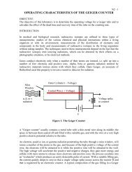
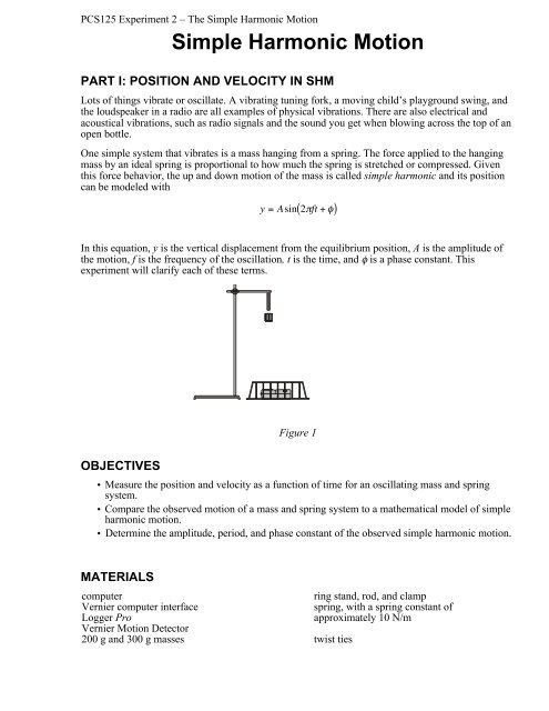
Figure 1<br />
OBJECTIVES<br />
• Measure the position and velocity as a function <strong>of</strong> time for an oscillat<strong>in</strong>g mass and spr<strong>in</strong>g<br />
system.<br />
• Compare the observed motion <strong>of</strong> a mass and spr<strong>in</strong>g system to a mathematical model <strong>of</strong> simple<br />
harmonic motion.<br />
• Determ<strong>in</strong>e the amplitude, period, and phase constant <strong>of</strong> the observed simple harmonic motion.<br />
MATERIALS<br />
computer<br />
r<strong>in</strong>g stand, rod, and clamp<br />
Vernier computer <strong>in</strong>terface<br />
Logger Pro<br />
Vernier <strong>Motion</strong> Detector<br />
spr<strong>in</strong>g, with a spr<strong>in</strong>g constant <strong>of</strong><br />
approximately 10 N/m<br />
200 g and 300 g masses twist ties
PCS125 Experiment 2 – The <strong>Simple</strong> <strong>Harmonic</strong> <strong>Motion</strong><br />
PRELIMINARY QUESTIONS<br />
1. Attach the 200 g mass to the spr<strong>in</strong>g and hold the free end <strong>of</strong> the spr<strong>in</strong>g <strong>in</strong> your hand, so the mass<br />
and spr<strong>in</strong>g hang down with the mass at rest. Lift the mass about 10 cm and release. Observe the<br />
motion. Sketch a graph <strong>of</strong> position vs. time for the mass.<br />
2. Just below the graph <strong>of</strong> position vs. time, and us<strong>in</strong>g the same length time scale, sketch a graph <strong>of</strong><br />
velocity vs. time for the mass.<br />
PROCEDURE<br />
1. Attach the spr<strong>in</strong>g to a horizontal rod connected to the vertical stand and hang the mass from the<br />
spr<strong>in</strong>g as shown <strong>in</strong> Figure 1. Securely fasten the 200 g mass to the spr<strong>in</strong>g and the spr<strong>in</strong>g to the<br />
rod, us<strong>in</strong>g twist ties so the mass cannot fall.<br />
2. Connect the <strong>Motion</strong> Detector to the DIG/SONIC 1 channel <strong>of</strong> the <strong>in</strong>terface.<br />
If the <strong>Motion</strong> Detector has a switch, set it to Normal.<br />
3. Place the <strong>Motion</strong> Detector at least 75 cm below the mass. Make sure there are no objects near<br />
the path between the detector and mass, such as a table edge.<br />
4. Open the file “15 <strong>Simple</strong> <strong>Harmonic</strong> <strong>Motion</strong>” from the <strong>Physics</strong> with Vernier folder.<br />
5. Make a prelim<strong>in</strong>ary run to make sure th<strong>in</strong>gs are set up correctly. Lift the mass upward a few<br />
centimeters and release. The mass should oscillate along a vertical l<strong>in</strong>e only. Click to<br />
beg<strong>in</strong> data collection.<br />
6. After 10 s, data collection will stop. The position graph should show a clean s<strong>in</strong>usoidal curve. If<br />
it has flat regions or spikes, reposition the <strong>Motion</strong> Detector and try aga<strong>in</strong>.<br />
7. Compare the position graph to your sketched prediction <strong>in</strong> the Prelim<strong>in</strong>ary Questions. How are<br />
the graphs similar How are they different Also, compare the velocity graph to your prediction.<br />
8. Measure the equilibrium position <strong>of</strong> the 200 g mass. To do this by allow the mass to hang free<br />
and at rest. Click to beg<strong>in</strong> data collection. After collection stops, click the Statistics<br />
button, , to determ<strong>in</strong>e the average distance from the detector. Record this distance as (y 0 ) <strong>in</strong><br />
your data table below.<br />
9. Now lift the mass upward about 5 cm and release it. The mass should oscillate along a vertical<br />
l<strong>in</strong>e only. Click to collect data. Exam<strong>in</strong>e the graphs. The pattern you are observ<strong>in</strong>g is<br />
characteristic <strong>of</strong> simple harmonic motion.<br />
10. Us<strong>in</strong>g the position graph, measure the time <strong>in</strong>terval between maximum positions. If you drag the<br />
mouse from one peak to another you can read along the x-axis the time <strong>in</strong>terval. This is the<br />
period, T, <strong>of</strong> the motion. The frequency, f, is the reciprocal <strong>of</strong> the period, f = 1/T. Based on your<br />
period measurement, calculate the frequency. Record the period, frequency and <strong>in</strong>itial phase<br />
constant <strong>of</strong> this motion <strong>in</strong> your data table (to f<strong>in</strong>d the <strong>in</strong>itial phase constant remember that a<br />
phase <strong>of</strong> π/2 would correspond to a quarter <strong>of</strong> a period).<br />
11. The amplitude, A, <strong>of</strong> simple harmonic motion is the maximum distance from the equilibrium<br />
position. Estimate values for the amplitude from your position graph. Enter the values <strong>in</strong> your<br />
data table.<br />
12. Repeat Steps 8–11 with the same 200 g mass, mov<strong>in</strong>g with larger amplitude than <strong>in</strong> the first run.<br />
13. Change the mass to 300 g and repeat Steps 8–11. Use an amplitude <strong>of</strong> about 5 cm. Store a good<br />
run made with this 300 g mass on the screen. You will use it for several <strong>of</strong> the Analysis<br />
questions.
PCS125 Experiment 2 – The <strong>Simple</strong> <strong>Harmonic</strong> <strong>Motion</strong><br />
DATA TABLE<br />
Run<br />
Mass<br />
(g)<br />
y 0<br />
(cm)<br />
A<br />
(cm)<br />
T<br />
(s)<br />
f<br />
(Hz)<br />
φ<br />
(rad)<br />
1<br />
2<br />
3<br />
ANALYSIS<br />
1. View the graphs <strong>of</strong> the last run on the screen. Compare the position vs. time and the velocity vs.<br />
time graphs. How are they the same How are they different<br />
2. Turn on the Exam<strong>in</strong>e mode by click<strong>in</strong>g the Exam<strong>in</strong>e button, . Move the mouse cursor back<br />
and forth across the graph to view the data values for the last run on the screen. Where is the<br />
mass when the velocity is zero Where is the mass when the velocity is maximum<br />
3. Does the frequency, f, appear to depend on the amplitude <strong>of</strong> the motion Do you have enough<br />
data to draw a firm conclusion<br />
4. Does the frequency, f, appear to depend on the mass used Did it change much <strong>in</strong> your tests<br />
5. You can compare your experimental data to the s<strong>in</strong>usoidal function model us<strong>in</strong>g the Manual<br />
Curve Fit feature <strong>of</strong> Logger Pro. Try it with your 300 g data. The model equation <strong>in</strong> the<br />
<strong>in</strong>troduction, which is similar to the one <strong>in</strong> many textbooks, gives the displacement from<br />
equilibrium. However, your <strong>Motion</strong> Detector reports the distance from the detector. To compare<br />
the model to your data, add the equilibrium distance to the model; that is, use<br />
y = y 0<br />
+ As<strong>in</strong>( 2πft + φ)<br />
where y 0 represents the equilibrium distance.<br />
a. Click once on the position € graph to select it.<br />
b. Choose Curve Fit from the Analyze menu.<br />
c. Select Manual as the Fit Type.<br />
d. Select the S<strong>in</strong>e function from the General Equation list.<br />
e. The S<strong>in</strong>e equation is <strong>of</strong> the form<br />
y=A*s<strong>in</strong>(Bt +C) + D.<br />
Compare this to the form <strong>of</strong> the equation above to match variables; e.g., φ corresponds to C, and<br />
2πf corresponds to B.<br />
f. Adjust the values for A, B and D to reflect your values for A, f and y 0 . You can either enter<br />
the values directly <strong>in</strong> the dialog box or you can use the up and down arrows to adjust the<br />
values.<br />
g. The phase parameter φ is called the phase constant and is used to adjust the y value reported<br />
by the model at t = 0 so that it matches your data. S<strong>in</strong>ce data collection did not necessarily<br />
beg<strong>in</strong> when the mass was at the equilibrium position, φ is needed to achieve a good match.<br />
h. The optimum value for φ will be between 0 and 2π. F<strong>in</strong>d a value for φ that makes the model<br />
come as close as possible to the data <strong>of</strong> your 300 g experiment. You may also want to adjust<br />
y 0 , A, and f to improve the fit. Write down the equation that best matches your data.<br />
6. Does the model fit the data well How can you tell
PCS125 Experiment 2 – The <strong>Simple</strong> <strong>Harmonic</strong> <strong>Motion</strong><br />
7. Predict what would happen to the plot <strong>of</strong> the model if you doubled the parameter for A by<br />
sketch<strong>in</strong>g both the current model and the new model with doubled A. Now double the parameter<br />
for A <strong>in</strong> the manual fit dialog box to compare to your prediction.<br />
8. Similarly, predict how the model plot would change if you doubled f, and then check by<br />
modify<strong>in</strong>g the model def<strong>in</strong>ition.<br />
9. Click , and optionally pr<strong>in</strong>t your graph.<br />
EXTENSIONS<br />
1. Investigate how chang<strong>in</strong>g the spr<strong>in</strong>g amplitude changes the period <strong>of</strong> the motion. Take care not<br />
to use too large amplitude so that the mass does not come closer than 40 cm to the detector or<br />
fall from the spr<strong>in</strong>g.<br />
2. How will damp<strong>in</strong>g change the data Tape an <strong>in</strong>dex card to the bottom <strong>of</strong> the mass and collect<br />
additional data. You may want to take data for about 2 m<strong>in</strong>utes. Does the model still fit well <strong>in</strong><br />
this case<br />
3. Describe how would you have to extend this experiment to discover the relationship between the<br />
mass attached to the spr<strong>in</strong>g and the period <strong>of</strong> his motion.<br />
PART II: ENERGY IN SHM<br />
We can describe an oscillat<strong>in</strong>g mass <strong>in</strong> terms <strong>of</strong> its position, velocity, and acceleration as a function<br />
<strong>of</strong> time. We can also describe the system from an energy perspective. In this experiment, you will<br />
measure the position and velocity as a function <strong>of</strong> time for an oscillat<strong>in</strong>g mass and spr<strong>in</strong>g system,<br />
and from those data, plot the k<strong>in</strong>etic and potential energies <strong>of</strong> the system.<br />
<strong>Energy</strong> is present <strong>in</strong> three forms for the mass and spr<strong>in</strong>g system. The mass m, with velocity v, can<br />
have k<strong>in</strong>etic energy KE<br />
The spr<strong>in</strong>g can hold elastic potential energy, or PE elastic . We calculate PE elastic by us<strong>in</strong>g<br />
where k is the spr<strong>in</strong>g constant and y is the extension or compression <strong>of</strong> the spr<strong>in</strong>g measured from the<br />
equilibrium position.<br />
The mass and spr<strong>in</strong>g system also has gravitational potential energy (PE gravitational = mgy), but we do<br />
not have to <strong>in</strong>clude the gravitational potential energy term if we measure the spr<strong>in</strong>g length from the<br />
hang<strong>in</strong>g equilibrium position. We can then concentrate on the exchange <strong>of</strong> energy between k<strong>in</strong>etic<br />
energy and elastic potential energy.<br />
If there are no other forces experienced by the system, then the pr<strong>in</strong>ciple <strong>of</strong> conservation <strong>of</strong> energy<br />
tells us that the sum ΔKE + ΔPE elastic = 0, which we can test experimentally.<br />
OBJECTIVES<br />
• Exam<strong>in</strong>e the energies <strong>in</strong>volved <strong>in</strong> simple harmonic motion.<br />
• Test the pr<strong>in</strong>ciple <strong>of</strong> conservation <strong>of</strong> energy.<br />
MATERIALS<br />
computer<br />
Vernier computer <strong>in</strong>terface<br />
slotted mass set, 50 g to 300 g <strong>in</strong> 50 g steps<br />
slotted mass hanger
PCS125 Experiment 2 – The <strong>Simple</strong> <strong>Harmonic</strong> <strong>Motion</strong><br />
Logger Pro<br />
spr<strong>in</strong>g, 1-10 N/m<br />
Vernier <strong>Motion</strong> Detector<br />
vertical stand<br />
wire basket<br />
PRELIMINARY QUESTIONS<br />
1. On the graphs <strong>of</strong> position velocity from part I, label the times when the spr<strong>in</strong>g has its greatest<br />
elastic potential energy. Then mark the times when it has the least elastic potential energy.<br />
2. Now try to sketch the graphs <strong>of</strong> k<strong>in</strong>etic energy vs. time and elastic potential energy vs. time.<br />
PROCEDURE<br />
1. The <strong>Motion</strong> Detector should still be connected to the DIG/SONIC 1 channel <strong>of</strong> the <strong>in</strong>terface and its<br />
switch set to Normal.<br />
2. To calculate the spr<strong>in</strong>g potential energy, it is necessary to measure the spr<strong>in</strong>g constant k. Hooke’s<br />
law states that the spr<strong>in</strong>g force is proportional to its extension from equilibrium, or<br />
F = –kx.<br />
You can apply a known force to the spr<strong>in</strong>g, to be balanced <strong>in</strong> magnitude by the spr<strong>in</strong>g force, by<br />
hang<strong>in</strong>g a range <strong>of</strong> weights from the spr<strong>in</strong>g. The <strong>Motion</strong> Detector can then be used to measure<br />
the equilibrium position. Open the experiment file “17b <strong>Energy</strong> <strong>in</strong> SHM.” Logger Pro is now set<br />
up to plot the applied weight vs. position.<br />
3. Click to beg<strong>in</strong> data collection. Hang a 50 g mass from the spr<strong>in</strong>g and allow the mass to<br />
hang motionless. Click and enter 0.49, the weight <strong>of</strong> the mass <strong>in</strong> newtons (N). Press<br />
ENTER to complete the entry. Now hang 100, 150, 200, 250, and 300 g from the spr<strong>in</strong>g,<br />
record<strong>in</strong>g the position and enter<strong>in</strong>g the weights <strong>in</strong> N. When you are done, click to end<br />
data collection.<br />
8. Click on the L<strong>in</strong>ear Fit button, , to fit a straight l<strong>in</strong>e to your data. The magnitude <strong>of</strong> the slope<br />
is the spr<strong>in</strong>g constant k <strong>in</strong> N/m. Record the value <strong>in</strong> the data table below.<br />
9. Open the experiment file “17c <strong>Energy</strong> <strong>in</strong> SHM.” In addition to plott<strong>in</strong>g position and velocity,<br />
three new data columns have been set up <strong>in</strong> this experiment file (k<strong>in</strong>etic energy, elastic potential<br />
energy, and the sum <strong>of</strong> these two <strong>in</strong>dividual energies). You may need to modify the calculations<br />
for the energies. Adjust the parameter for mass and spr<strong>in</strong>g constant as appropriate.<br />
10. With the mass hang<strong>in</strong>g from the spr<strong>in</strong>g and at rest, click to zero the <strong>Motion</strong> Detector.<br />
From now on, all distances will be measured relative to this position. When the mass moves<br />
closer to the detector, the position reported will be negative.<br />
12. Start the mass oscillat<strong>in</strong>g <strong>in</strong> a vertical direction only, with an amplitude <strong>of</strong> about 10 cm. Click<br />
to gather position, velocity, and energy data.<br />
DATA TABLE<br />
Spr<strong>in</strong>g constant<br />
N/m<br />
ANALYSIS<br />
1. Click on the y-axis label <strong>of</strong> the velocity graph to choose another column for plott<strong>in</strong>g. Click on<br />
More to see all <strong>of</strong> the columns. Uncheck the velocity column and select the k<strong>in</strong>etic energy and<br />
potential energy columns. Click to draw the new plot.
PCS125 Experiment 2 – The <strong>Simple</strong> <strong>Harmonic</strong> <strong>Motion</strong><br />
2. Compare your two energy plots to the sketches you made earlier. Be sure you compare to a<br />
s<strong>in</strong>gle cycle beg<strong>in</strong>n<strong>in</strong>g at the same po<strong>in</strong>t <strong>in</strong> the motion as your predictions. Comment on any<br />
differences.<br />
3. If mechanical energy is conserved <strong>in</strong> this system, how should the sum <strong>of</strong> the k<strong>in</strong>etic and<br />
potential energies vary with time Choose Draw Prediction from the Analyze menu and draw<br />
your prediction <strong>of</strong> this sum as a function <strong>of</strong> time.<br />
4. Check your prediction. Click on the y-axis label <strong>of</strong> the energy graph to choose another column<br />
for plott<strong>in</strong>g. Click on More and select the total energy column <strong>in</strong> addition to the other energy<br />
columns. Click to draw the new plot.<br />
5. From the shape <strong>of</strong> the total energy vs. time plot, what can you conclude about the conservation<br />
<strong>of</strong> mechanical energy <strong>in</strong> your mass and spr<strong>in</strong>g system<br />
EXTENSIONS<br />
1. In the <strong>in</strong>troduction, we claimed that the gravitational potential energy could be ignored if the<br />
displacement used <strong>in</strong> the elastic potential energy was measured from the hang<strong>in</strong>g equilibrium<br />
position. First write the total mechanical energy (k<strong>in</strong>etic, gravitational potential, and elastic<br />
potential energy) <strong>in</strong> terms <strong>of</strong> a coord<strong>in</strong>ate system, position measured upward and labeled y,<br />
whose orig<strong>in</strong> is located at the bottom <strong>of</strong> the relaxed spr<strong>in</strong>g <strong>of</strong> constant k (no force applied).<br />
2. Then determ<strong>in</strong>e the equilibrium position s when a mass m is suspended from the spr<strong>in</strong>g. This<br />
will be the new orig<strong>in</strong> for a coord<strong>in</strong>ate system with position labeled h. Write a new<br />
expression for total energy <strong>in</strong> terms <strong>of</strong> h. Show that when the energy is written <strong>in</strong> terms <strong>of</strong> h<br />
rather than y, the gravitational potential energy term cancels out.