Computer (matrix) version of the stiffness method 1. The computer ...
Computer (matrix) version of the stiffness method 1. The computer ...
Computer (matrix) version of the stiffness method 1. The computer ...

You also want an ePaper? Increase the reach of your titles
YUMPU automatically turns print PDFs into web optimized ePapers that Google loves.
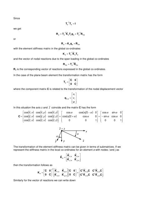
Since<br />
we get<br />
or<br />
T<br />
e<br />
T T = I<br />
~<br />
R +<br />
e<br />
T<br />
T<br />
e = Te<br />
KeTeqe<br />
Te<br />
R0e<br />
R = K q + R<br />
e e e 0e<br />
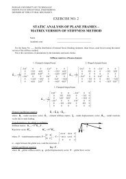
with <strong>the</strong> element <strong>stiffness</strong> <strong>matrix</strong> in <strong>the</strong> global co-ordinates<br />
and <strong>the</strong> vector <strong>of</strong> nodal reactions due to <strong>the</strong> span loading in <strong>the</strong> global co-ordinates<br />
T ~<br />
R = T R<br />
K<br />
e<br />
= T<br />
T<br />
e<br />
~<br />
K<br />
e<br />
T<br />
e<br />
0e e 0e<br />
R e is <strong>the</strong> corresponding vector <strong>of</strong> reactions expressed in <strong>the</strong> global co-ordinates.<br />
In <strong>the</strong> case <strong>of</strong> <strong>the</strong> plane beam element <strong>the</strong> transformation <strong>matrix</strong> has <strong>the</strong> form<br />
T e<br />
⎡C<br />
0⎤<br />
= ⎢ ⎥<br />
⎣0<br />
C⎦<br />
where <strong>the</strong> component <strong>matrix</strong> C is related to <strong>the</strong> transformation <strong>of</strong> <strong>the</strong> nodal displacement vector<br />
q<br />
n,<br />
e<br />
⎡ui<br />
⎤<br />
⎢ ⎥<br />
=<br />
⎢<br />
v i ⎥<br />
⎢⎣<br />
ϕ ⎥<br />
i ⎦<br />
In this situation <strong>the</strong> axis z and z ~ coincide and <strong>the</strong> <strong>matrix</strong> C has <strong>the</strong> form<br />
⎡cos<br />
⎢<br />
C = ⎢cos<br />
⎢<br />
⎣cos<br />
( x<br />
~ , x) cos( x<br />
~ , y ) cos( x<br />
~ , z)<br />
( y<br />
~ , x) cos( y<br />
~ , y ) cos( y<br />
~ , z)<br />
( z<br />
~ , x) cos( z<br />
~ , x) cos( z<br />
~ , z)<br />
⎤ ⎡ cosα<br />
⎥ ⎢<br />
⎥ =<br />
⎢<br />
cos<br />
⎥<br />
⎦<br />
⎢⎣<br />
0<br />
( π 2 + α )<br />
cos<br />
( π 2 − α )<br />
cosα<br />
0<br />
0⎤<br />
⎡ cosα<br />
⎥ ⎢<br />
0<br />
⎥<br />
=<br />
⎢<br />
− sinα<br />
1⎥⎦<br />
⎢⎣<br />
0<br />
sinα<br />
cosα<br />
0<br />
0⎤<br />
⎥<br />
0<br />
⎥<br />
1⎥⎦<br />
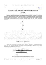
α<br />
y ~<br />
z ~ =<br />
z<br />
y<br />
α<br />
x ~<br />
x<br />
<strong>The</strong> transformation <strong>of</strong> <strong>the</strong> element <strong>stiffness</strong> <strong>matrix</strong> can be given in terms <strong>of</strong> submatrices. If we<br />
represent <strong>the</strong> <strong>stiffness</strong> <strong>matrix</strong> in <strong>the</strong> local co-ordinates for an element e with nodes i and j as<br />
<strong>the</strong>n <strong>the</strong> transformation follows as<br />
K<br />
e<br />
⎡C<br />
= ⎢<br />
⎣0<br />
0⎤<br />
⎥<br />
C⎦<br />
T<br />
⎡~<br />
K<br />
⎢~<br />
⎢⎣<br />
K<br />
ii,<br />
e<br />
ji,<br />
e<br />
~<br />
K<br />
e<br />
~<br />
K<br />
~<br />
K<br />
⎡~<br />
K<br />
= ⎢~<br />
⎢⎣<br />
K<br />
ij,<br />
e<br />
jj,<br />
e<br />
ii,<br />
e<br />
ji,<br />
e<br />
⎤⎡C<br />
⎥⎢<br />
⎥⎦<br />
⎣0<br />
Similarly for <strong>the</strong> vector <strong>of</strong> reactions we can write down<br />
~<br />
K<br />
~<br />
K<br />
ij,<br />
e<br />
jj,<br />
e<br />
⎤<br />
⎥<br />
⎥⎦<br />
⎡ T ~<br />
0⎤<br />
C K<br />
⎥ = ⎢<br />
T ~<br />
C⎦<br />
⎢⎣<br />
C K<br />
ii,<br />
e<br />
ji,<br />
e<br />
C<br />
C<br />
T ~<br />
C Kij<br />
T ~<br />
C K<br />
, e<br />
jj,<br />
e<br />
C⎤<br />
⎥<br />
C⎥⎦