Computer (matrix) version of the stiffness method 1. The computer ...
Computer (matrix) version of the stiffness method 1. The computer ...
Computer (matrix) version of the stiffness method 1. The computer ...

Create successful ePaper yourself
Turn your PDF publications into a flip-book with our unique Google optimized e-Paper software.
<strong>Computer</strong> (<strong>matrix</strong>) <strong>version</strong> <strong>of</strong> <strong>the</strong> <strong>stiffness</strong> <strong>method</strong><br />
<strong>1.</strong> <strong>The</strong> <strong>computer</strong> <strong>version</strong> <strong>of</strong> <strong>the</strong> <strong>stiffness</strong> <strong>matrix</strong> is a generalization <strong>of</strong> <strong>the</strong> classical <strong>version</strong> leading<br />
towards <strong>the</strong> <strong>computer</strong> applications and <strong>the</strong> finite element <strong>method</strong>. <strong>The</strong> basic ideas remain <strong>the</strong><br />
same, though some assumptions are released.<br />
<strong>The</strong> <strong>computer</strong> <strong>version</strong> is based on <strong>the</strong> following assumptions<br />
– displacements and strains remain small compared to <strong>the</strong> dimensions <strong>of</strong> <strong>the</strong> structure – <strong>the</strong><br />
equilibrium is related to <strong>the</strong> undeformed configuration (1 st order <strong>the</strong>ory)<br />
– material is linearly elastic with classical Hooke’s law<br />
– plane cross-sections remain plane during bending<br />
– from <strong>the</strong>se three conditions it follows that <strong>the</strong> superposition rule is valid<br />
Compared to <strong>the</strong> classical approach <strong>the</strong> assumption <strong>of</strong> no deformability in <strong>the</strong> axial direction <strong>of</strong> <strong>the</strong><br />
bars is released. Hence, <strong>the</strong> influence <strong>of</strong> <strong>the</strong> axial forces on <strong>the</strong> displacements is taken into<br />
account.<br />
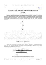
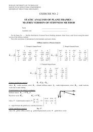
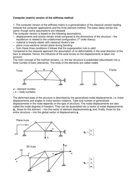
<strong>The</strong> main concept <strong>of</strong> <strong>the</strong> <strong>method</strong> remains, i.e. <strong>the</strong> bar structure is subdivided (discretised) into a<br />
finite number <strong>of</strong> bars (elements). <strong>The</strong> ends <strong>of</strong> <strong>the</strong> elements are called nodes.<br />
Truss<br />
i<br />
e<br />
k<br />
Frame<br />
e – element number<br />
i, k – node numbers<br />
<strong>The</strong> deformed state <strong>of</strong> <strong>the</strong> structure is described by <strong>the</strong> generalized nodal displacements, i.e. linear<br />
displacements and angles <strong>of</strong> cross-section rotations. Type and number <strong>of</strong> generalized<br />
displacements in <strong>the</strong> node depends on <strong>the</strong> type <strong>of</strong> structure. <strong>The</strong> nodal displacements are also<br />
called <strong>the</strong> nodal degrees <strong>of</strong> freedom. <strong>The</strong>y can be assembled into a vector <strong>of</strong> nodal displacements<br />
q n , those for <strong>the</strong> element – into <strong>the</strong> vector <strong>of</strong> element displacements q e and, finally, those for <strong>the</strong><br />
entire structure – into <strong>the</strong> global vector <strong>of</strong> displacements q.<br />
Plane truss<br />
y<br />
x<br />
i<br />
u i<br />
q<br />
n<br />
⎡ui<br />
⎤<br />
= ⎢ ⎥<br />
⎣v<br />
i ⎦<br />
v i<br />
z<br />
3D truss<br />
y<br />
u i<br />
i<br />
w i<br />
v i<br />
x<br />
q<br />
n<br />
⎡ui<br />
⎢<br />
=<br />
⎢<br />
v i<br />
⎢⎣<br />
wi<br />
⎤<br />
⎥<br />
⎥<br />
⎥⎦
Plane frame<br />
x<br />
i<br />
v i<br />
u i<br />
q<br />
n<br />
⎡ui<br />
⎤<br />
⎢ ⎥<br />
=<br />
⎢<br />
v i ⎥<br />
⎢⎣<br />
ϕ ⎥<br />
i ⎦<br />
y<br />
x<br />
z<br />
3D frame<br />
y<br />
u i<br />
ϕ x<br />
ϕ z<br />
ϕ i<br />
i<br />
w i<br />
v i<br />
ϕ x<br />
ϕ y<br />
Plane yz<br />
q<br />
n<br />
⎡ui<br />
⎤<br />
⎢ ⎥<br />
⎢<br />
v i ⎥<br />
⎢w<br />
⎥<br />
i<br />
= ⎢ ⎥<br />
⎢ϕ<br />
x ⎥<br />
⎢ϕ<br />
⎥<br />
y<br />
⎢ ⎥<br />
⎢⎣<br />
ϕz<br />
⎥⎦<br />
Interpretation<br />
<strong>of</strong> <strong>the</strong> rotation angle<br />
<strong>The</strong> displacements presented in <strong>the</strong> above figures are referred to <strong>the</strong> global sets <strong>of</strong> co-ordinates xy<br />
or xyz. In practice it is much easier to form <strong>the</strong> basic equations on <strong>the</strong> level <strong>of</strong> elements, hence, <strong>the</strong><br />
local systems <strong>of</strong> co-ordinates are introduced. <strong>The</strong> values corresponding to <strong>the</strong> local co-ordinates<br />
are additionally denoted with tildes.<br />
<strong>The</strong> slope-defection formulae from <strong>the</strong> classical <strong>stiffness</strong> <strong>method</strong> are replaced by <strong>the</strong> element<br />
<strong>stiffness</strong> <strong>matrix</strong>, which relates <strong>the</strong> element displacements in local co-ordinates to <strong>the</strong> reactions at<br />
<strong>the</strong> element supports in local co-ordinates:<br />
~ K<br />
~ ~<br />
Re<br />
= Keq<br />
~<br />
e e<br />
[ k eij<br />
]<br />
n×<br />
n<br />
where n is <strong>the</strong> number <strong>of</strong> element degrees <strong>of</strong> freedom. <strong>The</strong> elements <strong>of</strong> <strong>the</strong> <strong>stiffness</strong> <strong>matrix</strong><br />
represent reactions at <strong>the</strong> element supports created by unit displacements. For instance, <strong>the</strong><br />
element k ~ eij represents <strong>the</strong> reaction number i created by <strong>the</strong> action <strong>of</strong> <strong>the</strong> displacement q<br />
~ = j 1<br />
First, let us consider <strong>the</strong> plane truss element. In this case <strong>the</strong> vectors <strong>of</strong> element displacements<br />
and reactions have four components<br />
= ~<br />
~ q<br />
~<br />
i<br />
R 1,<br />
1<br />
2<br />
~ R 3,<br />
q<br />
~<br />
3<br />
x ~<br />
k<br />
e<br />
~ ~<br />
l<br />
R 4,<br />
q 4<br />
~ R<br />
~<br />
2,<br />
q<br />
y ~<br />
q<br />
~<br />
e<br />
⎡u<br />
~ ⎤ ⎡ ~<br />
i q1<br />
⎤<br />
⎢ ⎥ ⎢ ⎥<br />
⎢v<br />
~ ~<br />
i ⎥ = ⎢q2<br />
= ⎥<br />
⎢u<br />
~ ⎥ ⎢~<br />
⎥<br />
k q3<br />
⎢ ⎥ ⎢~<br />
⎥<br />
~<br />
⎣v<br />
k<br />
⎦ ⎢⎣<br />
q4<br />
⎥⎦<br />
~<br />
R<br />
e<br />
⎡ ~<br />
R<br />
⎢ ~<br />
⎢R<br />
=<br />
⎢ ~<br />
R<br />
⎢ ~<br />
⎢⎣<br />
R<br />
1<br />
2<br />
3<br />
4<br />
⎤ ⎡−<br />
Ni<br />
⎤<br />
⎥ ⎢ ⎥<br />
⎥ ⎢<br />
−Ti<br />
= ⎥<br />
⎥ ⎢ N ⎥<br />
k<br />
⎥ ⎢ ⎥<br />
⎥⎦<br />
⎣ Tk<br />
⎦
N<br />
State q ~<br />
1<br />
1 =<br />
e<br />
i<br />
q ~<br />
y ~<br />
1 =<br />
1<br />
k<br />
N<br />
x ~<br />
From <strong>the</strong> Hooke’s law<br />
EA ~ EA ~<br />
N = − ⋅1<br />
⇒ R1<br />
= , R3<br />
l<br />
l<br />
EA<br />
= −<br />
l<br />
State q ~<br />
1<br />
i<br />
N<br />
3 =<br />
e<br />
k<br />
N<br />
q ~<br />
3 = 1<br />
x ~<br />
From <strong>the</strong> Hooke’s law<br />
EA ~ EA ~ EA<br />
N = ⋅1<br />
⇒ R1<br />
= − , R3<br />
=<br />
l<br />
l l<br />
y ~<br />
State<br />
~<br />
1<br />
i<br />
q y ~ x ~<br />
2 =<br />
e<br />
k<br />
x ~<br />
No internal forces are created. <strong>The</strong> same<br />
situation occurs in <strong>the</strong> state q ~<br />
1 .<br />
4 =<br />
q ~<br />
2 =<br />
1<br />
y ~<br />
Summarising <strong>of</strong> <strong>the</strong>se results yields <strong>the</strong> following element <strong>stiffness</strong> <strong>matrix</strong><br />
~<br />
K<br />
e<br />
⎡ 1<br />
⎢<br />
EA ⎢<br />
0<br />
=<br />
l ⎢−1<br />
⎢<br />
⎣ 0<br />
From <strong>the</strong> physical interpretation <strong>of</strong> <strong>the</strong> element <strong>stiffness</strong> <strong>matrix</strong> it follows, that for instance <strong>the</strong> first<br />
column <strong>of</strong> this <strong>matrix</strong> represents <strong>the</strong> vector <strong>of</strong> reactions in <strong>the</strong> element created by <strong>the</strong> action <strong>of</strong> <strong>the</strong><br />
displacement q ~<br />
1 .<br />
1 =<br />
Now, let us consider <strong>the</strong> <strong>stiffness</strong> <strong>matrix</strong> for <strong>the</strong> plane bar element under bending (i.e. <strong>the</strong> plane<br />
beam element).<br />
~ R 4,<br />
q<br />
~<br />
4<br />
k<br />
⎡u<br />
~ ⎤ ⎡q<br />
~ ⎤ ⎡ ~<br />
i 1 R ⎤ ⎡−<br />
N ⎤<br />
1<br />
ik<br />
e<br />
~ ⎢ ~ ⎥ ⎢~<br />
⎥ ⎢ ~ ⎥ ⎢ ⎥<br />
R<br />
⎢v<br />
i ⎥ ⎢q2<br />
⎥ ⎢R<br />
⎥ ⎢<br />
−T<br />
6,<br />
q<br />
~<br />
6<br />
2 ik ⎥<br />
~ ⎢ ~ ⎥ ⎢~<br />
~ ϕ q ⎥ ⎢ ~<br />
R<br />
i<br />
⎥ ⎢<br />
i 3<br />
M ⎥<br />
1,<br />
q<br />
~<br />
l<br />
1<br />
~ ~ R3<br />
ik<br />
R q e = ⎢~<br />
⎥ = ⎢~<br />
⎥ R e = ⎢ ⎥ = ⎢ ⎥<br />
5,<br />
q<br />
~<br />
5<br />
~<br />
⎢uk<br />
⎥ ⎢q4<br />
⎥ ⎢R<br />
⎥ ⎢ N<br />
4 ki ⎥<br />
~ ⎢v<br />
~ ⎥ ⎢q<br />
~ ⎥ ⎢ ~<br />
~<br />
⎥ ⎢ ⎥<br />
k 5<br />
Tki<br />
⎢ ⎥ ⎢<br />
~<br />
⎥ ⎢<br />
R5<br />
~ R 2,<br />
q 2<br />
⎥<br />
⎢<br />
~<br />
~ ⎢ ⎥<br />
R 3,<br />
q<br />
~<br />
3<br />
⎣ϕ<br />
k ⎥⎦<br />
⎢⎣<br />
q6<br />
⎥⎦<br />
⎢⎣<br />
R ⎥⎦<br />
⎢⎣<br />
M<br />
6 ki ⎥⎦<br />
0<br />
0<br />
0<br />
0<br />
−1<br />
0<br />
1<br />
0<br />
0⎤<br />
⎥<br />
0<br />
⎥<br />
0⎥<br />
⎥<br />
0⎦
Reactions number 1 and 4 created by <strong>the</strong> action <strong>of</strong> displacements number 1 and 4 are obtained in<br />
<strong>the</strong> same way as in <strong>the</strong> case <strong>of</strong> <strong>the</strong> plane truss element. Note, that <strong>the</strong>se displacements do not<br />
yield any o<strong>the</strong>r reactions. Also, <strong>the</strong>se reactions are zero under <strong>the</strong> action <strong>of</strong> all <strong>the</strong> o<strong>the</strong>r<br />
displacements. Hence, in <strong>the</strong> classical plane beam element <strong>the</strong> action <strong>of</strong> axial forces and<br />
displacements is fully decoupled from <strong>the</strong> combined action <strong>of</strong> shear and bending. <strong>The</strong> reactions<br />
due to <strong>the</strong> transverse displacements and cross-section rotations can be found using <strong>the</strong> slopedeflection<br />
formulae from <strong>the</strong> classical <strong>stiffness</strong> <strong>method</strong>. This yields:<br />
~<br />
R<br />
3<br />
~<br />
R<br />
6<br />
~<br />
R<br />
2<br />
~<br />
R<br />
5<br />
2EI<br />
= M =<br />
ψ<br />
l<br />
2EI<br />
⎛<br />
l ⎝<br />
6EI<br />
4EI<br />
l<br />
6EI<br />
5 2<br />
( 2ϕ<br />
)<br />
~ ~<br />
~ ~ ~ ~<br />
i + ϕk<br />
− 3 ik = ⎜2q3<br />
+ q6<br />
− 3 ⎟ = q2<br />
+ q3<br />
− q5<br />
q6<br />
ik +<br />
2<br />
2<br />
2EI<br />
= M =<br />
ψ<br />
l<br />
2EI<br />
⎛<br />
l ⎝<br />
q<br />
~<br />
− q<br />
~<br />
⎞<br />
l ⎠<br />
l<br />
6EI<br />
2EI<br />
l<br />
l<br />
6EI<br />
2EI<br />
l<br />
5 2<br />
( 2ϕ<br />
)<br />
~ ~<br />
~ ~ ~ ~<br />
k + ϕi<br />
− 3 ik = ⎜2q6<br />
+ q3<br />
− 3 ⎟ = q2<br />
+ q3<br />
− q5<br />
q6<br />
ki +<br />
2<br />
2<br />
6EI<br />
= −T<br />
=<br />
ψ<br />
l<br />
6EI<br />
⎛<br />
q<br />
~<br />
− q<br />
~<br />
⎞<br />
l ⎠<br />
l<br />
12EI<br />
6EI<br />
l<br />
12EI<br />
4EI<br />
l<br />
5 2<br />
( ϕ<br />
)<br />
~ ~<br />
~ ~ ~ ~<br />
i + ϕk<br />
− 2 ik = ⎜q3<br />
+ q6<br />
− 2 ⎟ = q2<br />
+ q3<br />
− q5<br />
q6<br />
ik +<br />
2<br />
2<br />
3<br />
2<br />
3<br />
6EI<br />
6EI<br />
⎛<br />
= T ( )<br />
~<br />
ki = − ϕ<br />
2 i + ϕk<br />
− 2ψ<br />
ik = − ⎜q<br />
2<br />
l<br />
l ⎝<br />
12EI<br />
~ 6EI<br />
~ 12EI<br />
~ 6EI<br />
= − q<br />
~<br />
3 2 − q<br />
2 3 + q<br />
3 5 − q<br />
2<br />
l l l l<br />
l<br />
⎝<br />
3<br />
6<br />
+ q<br />
~<br />
6<br />
q<br />
~<br />
q<br />
~<br />
− 2<br />
− q<br />
~<br />
⎞<br />
l ⎠<br />
Summarising <strong>the</strong>se calculations yield <strong>the</strong> following <strong>stiffness</strong> <strong>matrix</strong> for <strong>the</strong> plane beam element<br />
~<br />
K<br />
e<br />
⎡<br />
⎢<br />
⎢<br />
⎢ 0<br />
⎢<br />
⎢<br />
⎢ 0<br />
= ⎢<br />
⎢−<br />
⎢<br />
⎢<br />
⎢<br />
⎢<br />
⎢<br />
⎣<br />
EA<br />
l<br />
EA<br />
l<br />
0<br />
0<br />
12EI<br />
l<br />
6EI<br />
l<br />
12EI<br />
−<br />
3<br />
l<br />
6EI<br />
l<br />
0<br />
3<br />
2<br />
0<br />
2<br />
0<br />
6EI<br />
2<br />
l<br />
4EI<br />
l<br />
0<br />
6EI<br />
−<br />
2<br />
l<br />
2EI<br />
l<br />
5<br />
− q<br />
~<br />
l<br />
−<br />
2<br />
EA<br />
l<br />
0<br />
0<br />
EA<br />
l<br />
0<br />
0<br />
⎞<br />
⎟<br />
⎠<br />
=<br />
l<br />
0<br />
12EI<br />
−<br />
3<br />
l<br />
6EI<br />
−<br />
2<br />
l<br />
0<br />
12EI<br />
3<br />
l<br />
6EI<br />
−<br />
2<br />
l<br />
l<br />
⎤<br />
0 ⎥<br />
6EI<br />
⎥<br />
⎥<br />
2<br />
l ⎥<br />
2EI<br />
⎥<br />
l ⎥<br />
⎥<br />
0 ⎥<br />
⎥<br />
6EI<br />
⎥<br />
−<br />
2<br />
l<br />
⎥<br />
4EI<br />
⎥<br />
⎥<br />
l ⎦<br />
It is worth to note, that <strong>the</strong> element <strong>stiffness</strong> matrices are symmetric. This is <strong>the</strong> consequence <strong>of</strong><br />
<strong>the</strong> reactions reciprocity <strong>the</strong>orem (Rayleigh’s <strong>the</strong>orem) stating that<br />
k ij = k ji<br />
<strong>The</strong> physical interpretation <strong>of</strong> <strong>the</strong> entries in this <strong>matrix</strong> is unchanged, i.e. for instance <strong>the</strong> second<br />
column collects <strong>the</strong> values <strong>of</strong> reactions created by <strong>the</strong> action <strong>of</strong> <strong>the</strong> displacement q ~<br />
1 .<br />
After <strong>the</strong> derivation <strong>of</strong> <strong>the</strong>se two examples <strong>of</strong> <strong>the</strong> element <strong>stiffness</strong> matrices let us now deal with<br />
<strong>the</strong> loading. Generally, <strong>the</strong> loading is split into actions directly at <strong>the</strong> nodes and <strong>the</strong> actions along<br />
<strong>the</strong> elements. <strong>The</strong> former one will be considered at <strong>the</strong> later stages. <strong>The</strong> latter one must be<br />
transferred to <strong>the</strong> nodes in <strong>the</strong> form <strong>of</strong> appropriate reactions. <strong>The</strong>y are assembled into a vector <strong>of</strong><br />
reactions due to <strong>the</strong> span loading<br />
~<br />
R<br />
~<br />
[ R0<br />
i<br />
] 1,2,..., 6<br />
0 e =<br />
6× 1<br />
i =<br />
This vector enters <strong>the</strong> equation <strong>of</strong> element equilibrium as an additional term<br />
l<br />
2 =<br />
6EI<br />
l<br />
2
~ ~ ~ ~<br />
R = K q + R<br />
e e e 0e<br />
For instance, in <strong>the</strong> case <strong>of</strong> <strong>the</strong> uniformly distributed load on <strong>the</strong> beam we have<br />
~<br />
R01<br />
~<br />
R03<br />
i<br />
~<br />
R04<br />
x ~<br />
k ~<br />
R06<br />
e<br />
l ~<br />
R05<br />
~<br />
R02<br />
y ~<br />
~<br />
R<br />
0e<br />
⎡ ~<br />
R<br />
⎢ ~<br />
⎢R<br />
⎢ ~<br />
R<br />
= ⎢ ~<br />
⎢R<br />
⎢ ~<br />
⎢<br />
R<br />
~<br />
⎢⎣<br />
R<br />
01<br />
02<br />
03<br />
04<br />
05<br />
06<br />
⎡ 0 ⎤<br />
⎤ ⎢ ql ⎥<br />
⎢ −<br />
⎥ 2<br />
⎥<br />
⎥ ⎢ 2 ⎥<br />
⎢ ql<br />
⎥ − ⎥<br />
⎥ = ⎢ ⎥<br />
⎥ ⎢ 0 12 ⎥<br />
⎥ ⎢ ql ⎥<br />
⎢ −<br />
⎥ ⎥<br />
⎥ ⎢<br />
2<br />
2 ⎥<br />
⎦ ⎢ ql ⎥<br />
⎢⎣<br />
12 ⎥⎦<br />
and in <strong>the</strong> case <strong>of</strong> <strong>the</strong> non-uniform heating ∆t with warmer upper side and <strong>the</strong> uniform heating t 0<br />
~<br />
R01<br />
~<br />
R03<br />
i<br />
~<br />
R04<br />
x ~<br />
∆t<br />
+<br />
t<br />
k<br />
0<br />
~<br />
–<br />
R06<br />
e l ~<br />
R05<br />
~<br />
R02<br />
y ~<br />
~<br />
R<br />
0e<br />
⎡ ~<br />
R<br />
⎢ ~<br />
⎢R<br />
⎢ ~<br />
R<br />
= ⎢ ~<br />
⎢R<br />
⎢ ~<br />
⎢<br />
R<br />
~<br />
⎢⎣<br />
R<br />
01<br />
02<br />
03<br />
04<br />
05<br />
06<br />
⎤ ⎡ EAαtt0<br />
⎤<br />
⎥ ⎢ ⎥<br />
⎢<br />
0<br />
⎥<br />
⎥<br />
⎢<br />
∆t<br />
⎥ EIα<br />
⎥<br />
t<br />
⎥ = ⎢ ⎥<br />
⎥ ⎢ − EAα<br />
h tt0<br />
⎥<br />
⎥ ⎢ ⎥<br />
⎥ ⎢<br />
0<br />
⎥<br />
⎢<br />
∆t<br />
⎥ − ⎥<br />
⎦<br />
EIαt<br />
⎢⎣<br />
h ⎥⎦<br />
In <strong>the</strong> latter case note that <strong>the</strong> distribution <strong>of</strong> <strong>the</strong> bending moment is constant with <strong>the</strong> fibres under<br />
tension on <strong>the</strong> colder side. Hence, <strong>the</strong> shear force is zero leading to zero reactions number 2 and<br />
5. On <strong>the</strong> o<strong>the</strong>r hand, <strong>the</strong> uniform heating leads to <strong>the</strong> constant compressive axial force.<br />
To obtain <strong>the</strong> <strong>stiffness</strong> matrices for ano<strong>the</strong>r types <strong>of</strong> beams with degenerate supports, e.g. <strong>the</strong><br />
clamped-hinged beam, <strong>the</strong> clamped-slider beam, etc. <strong>the</strong> process <strong>of</strong> static condensation can be<br />
used.<br />
In general, <strong>the</strong> process uses <strong>the</strong> fact, that some reactions in <strong>the</strong> degenerate supports are zero. In<br />
<strong>the</strong> case <strong>of</strong> <strong>the</strong> hinge <strong>the</strong> moment is zero. From this condition <strong>the</strong> corresponding displacements<br />
can be eliminated and <strong>the</strong> dimension <strong>of</strong> <strong>the</strong> <strong>matrix</strong> is reduced from 6 by a number <strong>of</strong> zero reaction.<br />
<strong>The</strong> equilibrium conditions can be rearranged as:<br />
⎡~<br />
R<br />
⎢~<br />
⎢⎣<br />
R<br />
e1<br />
ec<br />
⎤ ⎡~<br />
K<br />
⎥ = ⎢~<br />
⎥⎦<br />
⎢⎣<br />
K<br />
and <strong>the</strong> reactions in degenerate supports<br />
~ ~ ~ ~<br />
R = K q + R<br />
e e e 0e<br />
e11<br />
ec1<br />
~<br />
K<br />
~<br />
K<br />
e1c<br />
ecc<br />
~<br />
R ec = 0<br />
⎤⎡q<br />
~<br />
⎥⎢~<br />
⎥⎦<br />
⎣q<br />
e1<br />
ec<br />
⎤ ⎡~<br />
R<br />
⎥ + ⎢~<br />
⎦ ⎢⎣<br />
R<br />
0e1<br />
0ec<br />
⎤<br />
⎥<br />
⎥⎦
⎪⎧<br />
~ ~ ~<br />
Re1<br />
= Ke11q<br />
~<br />
e1<br />
+ Ke1c<br />
q<br />
~<br />
⎨ ~ ~<br />
⎪⎩ 0 = K<br />
~<br />
ec1qe1<br />
+ K<br />
~<br />
eccqec<br />
From <strong>the</strong> second equation vector <strong>of</strong> displacements<br />
can be substituted into <strong>the</strong> first equation<br />
to get<br />
~<br />
R<br />
e1<br />
ec<br />
~<br />
+ R<br />
~<br />
+ R<br />
0e1<br />
0ec<br />
~<br />
( Kec1q<br />
~<br />
e1<br />
R ec )<br />
~ −1 ~<br />
ec = −Kecc<br />
0<br />
q<br />
~<br />
+<br />
e11<br />
e1<br />
e1c<br />
−1<br />
ecc<br />
~ ~ ~<br />
( K<br />
~<br />
ec1qe1<br />
+ R0ec<br />
) R0e1<br />
~ ~ ~ ~ ~<br />
R = K q − K K<br />
+<br />
=<br />
~ ~ ~ −1~<br />
( )<br />
~ ~ ~ ~ −1~<br />
Ke11<br />
− Ke1cK<br />
ecc Kec1<br />
qe1<br />
+ ( R0e1<br />
− Ke1cK<br />
ecc R ec )<br />
e1<br />
0<br />
where <strong>the</strong> expressions in <strong>the</strong> paren<strong>the</strong>ses are <strong>the</strong> modified <strong>stiffness</strong> <strong>matrix</strong> and <strong>the</strong> modified vector<br />
<strong>of</strong> reactions due to loading, respectively.<br />
~ ~ ~ ~ −1~<br />
Ke'<br />
= Ke11<br />
− Ke1cK<br />
ecc Kec1<br />
~ ~ ~ ~ −1~<br />
R ' = R − K K R<br />
So we have<br />
0e<br />
0e1<br />
e1c<br />
ecc<br />
~ ~ ~ ~<br />
R = K ' q + R<br />
e1 e e1<br />
0e<br />
<strong>The</strong> static condensation is very simple if just one displacement at a time is eliminated using <strong>the</strong><br />
single condition <strong>of</strong> <strong>the</strong> zero reaction. For instance if <strong>the</strong> displacement q ~ r is eliminated, <strong>the</strong>n<br />
'<br />
0ec<br />
⎧~<br />
~ ⎪k<br />
K e':<br />
⎨<br />
⎪~<br />
⎩k<br />
ln<br />
ln<br />
' = k<br />
~<br />
' = 0<br />
ln<br />
− k<br />
~<br />
for<br />
lr<br />
~<br />
~ 1 krn<br />
for l ≠ r<br />
krr<br />
l = r or n = r<br />
and<br />
n ≠ r<br />
~<br />
R<br />
0e<br />
⎧ ~<br />
⎪R<br />
': ⎨<br />
⎪ ~<br />
⎩R<br />
0l<br />
0l<br />
' = R<br />
~<br />
' = 0<br />
0l<br />
− k<br />
~ ~<br />
lr ~ 1 R<br />
krr<br />
for l = r<br />
0r<br />
for<br />
l<br />
≠ r<br />
So schematically we have<br />
n<br />
r<br />
n<br />
r<br />
l<br />
k ~<br />
ln<br />
k ~<br />
lr<br />
~<br />
R 0l<br />
l<br />
~<br />
k ln<br />
'<br />
0<br />
0<br />
~<br />
R 0l<br />
'<br />
0<br />
r<br />
k ~<br />
rn<br />
k ~<br />
rr<br />
~<br />
R 0r<br />
r<br />
0 0 0 0 0<br />
0<br />
0<br />
In <strong>the</strong> case <strong>of</strong> static reduction <strong>of</strong> several displacements this can be carried out step by step, one<br />
displacement after ano<strong>the</strong>r.<br />
For <strong>the</strong> clamped-hinged elements we have:
~ q<br />
~<br />
~<br />
K ' =<br />
e<br />
⎡<br />
⎢<br />
⎢<br />
⎢<br />
⎢<br />
⎢<br />
⎢<br />
⎢<br />
⎢−<br />
⎢<br />
⎢<br />
⎢<br />
⎢<br />
⎣<br />
EA<br />
l<br />
0<br />
0<br />
EA<br />
l<br />
0<br />
0<br />
i<br />
R 1,<br />
1<br />
2<br />
~ R , q<br />
~<br />
3<br />
3<br />
~ R 4,<br />
q<br />
~<br />
x ~<br />
~<br />
4<br />
R 4,<br />
q<br />
~<br />
4<br />
x<br />
k<br />
~<br />
k<br />
~<br />
~<br />
R<br />
e<br />
R 6 = 0<br />
6,<br />
q<br />
~<br />
6<br />
e<br />
~ ~ i<br />
~ R<br />
~<br />
R<br />
5,<br />
q<br />
1,<br />
q 1<br />
~<br />
5<br />
R 5,<br />
q<br />
~<br />
5<br />
~ R<br />
~<br />
2,<br />
q<br />
~ R<br />
~<br />
2,<br />
q<br />
R ~<br />
2<br />
3 = 0<br />
y ~ y ~<br />
0<br />
3EI<br />
3<br />
l<br />
3EI<br />
2<br />
l<br />
0<br />
3EI<br />
−<br />
3<br />
l<br />
0<br />
0<br />
3EI<br />
2<br />
l<br />
3EI<br />
l<br />
0<br />
6EI<br />
−<br />
2<br />
l<br />
0<br />
−<br />
EA<br />
l<br />
0<br />
0<br />
EA<br />
l<br />
0<br />
0<br />
0<br />
3EI<br />
−<br />
3<br />
l<br />
3EI<br />
−<br />
2<br />
l<br />
0<br />
3EI<br />
3<br />
l<br />
0<br />
⎤<br />
0⎥<br />
⎥<br />
0⎥<br />
⎥<br />
⎥<br />
0<br />
⎥<br />
⎥<br />
0⎥<br />
⎥<br />
⎥<br />
0<br />
⎥<br />
0⎥<br />
⎦<br />
~<br />
K<br />
⎡ EA<br />
⎢ l<br />
⎢<br />
⎢ 0<br />
⎢<br />
⎢ 0<br />
' = ⎢ EA<br />
⎢<br />
−<br />
l<br />
⎢<br />
⎢ 0<br />
⎢<br />
⎢<br />
⎢<br />
0<br />
⎣<br />
Example<br />
Elimination <strong>of</strong> q<br />
~<br />
3 in <strong>the</strong> case <strong>of</strong> <strong>the</strong> hinged-clamped beam.<br />
Let us check <strong>the</strong> value k 52 ' (l = 5, n = 2, r = 3)<br />
~<br />
k<br />
52<br />
' = k<br />
~<br />
52<br />
− k<br />
~<br />
53<br />
~<br />
~ 1 k<br />
k<br />
33<br />
32<br />
e<br />
12EI<br />
− 6EI<br />
1<br />
= − − ⋅<br />
3 2<br />
l l 4EI<br />
l<br />
0<br />
3EI<br />
3<br />
l<br />
0<br />
0<br />
3EI<br />
−<br />
3<br />
l<br />
3EI<br />
2<br />
l<br />
6EI<br />
⋅<br />
2<br />
l<br />
0<br />
0<br />
0<br />
0<br />
0<br />
0<br />
−<br />
3EI<br />
= −<br />
3<br />
l<br />
~<br />
Let us also calculate R ' for <strong>the</strong> case <strong>of</strong> point load at <strong>the</strong> beam centre (l = 6, r = 3)<br />
06<br />
EA<br />
l<br />
0<br />
0<br />
EA<br />
l<br />
0<br />
0<br />
0<br />
3EI<br />
−<br />
3<br />
l<br />
0<br />
0<br />
3EI<br />
3<br />
l<br />
3EI<br />
−<br />
2<br />
l<br />
⎤<br />
0 ⎥<br />
3EI<br />
⎥<br />
⎥<br />
2<br />
l ⎥<br />
0 ⎥<br />
⎥<br />
0<br />
⎥<br />
3EI<br />
⎥<br />
− ⎥<br />
2<br />
l ⎥<br />
3EI<br />
⎥<br />
l ⎥⎦<br />
~<br />
R<br />
03<br />
Pl<br />
= −<br />
8<br />
~ Pl<br />
R 06 =<br />
8<br />
R ~<br />
03 ' = 0<br />
~<br />
R<br />
06<br />
'<br />
~ ~ ~ ~ 2 1 3<br />
~ 1 Pl EI ⎛ Pl ⎞ Pl<br />
R 06'<br />
= R06<br />
− k36<br />
R03<br />
= − ⋅ ⋅ ⎜ − ⎟ =<br />
k 8 l 4EI<br />
8 16<br />
33<br />
⎝ ⎠<br />
l<br />
<strong>The</strong> 2D beam can be generalised to <strong>the</strong> 3D case. To this end we must include bending and shear<br />
in two planes as well as torsion.<br />
~ R 9,<br />
q<br />
~<br />
9<br />
z ~<br />
~<br />
x ~<br />
R 8,<br />
q<br />
~<br />
~<br />
k<br />
~<br />
8 R<br />
R<br />
~<br />
12,<br />
q<br />
~<br />
12<br />
7,<br />
q 7<br />
~<br />
~ ~<br />
R R 3,<br />
q<br />
11,<br />
q<br />
~<br />
11<br />
3<br />
~ e<br />
y ~ ~<br />
~ i<br />
R 10,<br />
q<br />
~<br />
10<br />
2,<br />
q ~<br />
2 R<br />
~<br />
6,<br />
q 6<br />
~ ~<br />
~ R<br />
~ R<br />
1,<br />
q<br />
5,<br />
q 5<br />
1 ~ R , q<br />
~<br />
R<br />
4 4
<strong>The</strong> complete <strong>stiffness</strong> <strong>matrix</strong> for <strong>the</strong> 3D beam has <strong>the</strong> following form<br />
⎡ EA<br />
EA<br />
⎢ 0 0 0 0 0 − 0 0<br />
l<br />
l<br />
⎢<br />
12EI<br />
⎢<br />
z<br />
6EIz<br />
−12EIz<br />
0 0 0<br />
0<br />
0<br />
3<br />
2<br />
3<br />
⎢ l<br />
l<br />
l<br />
⎢<br />
12EI<br />
y 6EIy<br />
−12EIy<br />
⎢<br />
0<br />
0 0 0<br />
3<br />
2<br />
3<br />
⎢<br />
l<br />
l<br />
l<br />
⎢<br />
GIs<br />
0 0 0 0 0<br />
⎢<br />
l<br />
⎢<br />
4EIy<br />
− 6EI<br />
y<br />
⎢<br />
0 0 0<br />
⎢<br />
l<br />
2<br />
l<br />
⎢<br />
4EIz<br />
− 6EIz<br />
⎢<br />
0<br />
0<br />
~<br />
=<br />
l<br />
2<br />
K ⎢<br />
l<br />
e'<br />
0<br />
⎢<br />
EA<br />
0 0<br />
⎢<br />
l<br />
⎢<br />
12EIz<br />
⎢<br />
0<br />
3<br />
⎢<br />
l<br />
⎢<br />
12EIy<br />
⎢<br />
3<br />
l<br />
⎢<br />
⎢ s y m m e t r y<br />
⎢<br />
⎢<br />
⎢<br />
⎢<br />
⎢<br />
⎣<br />
0<br />
0<br />
0<br />
− GI<br />
l<br />
0<br />
0<br />
0<br />
0<br />
0<br />
GI<br />
l<br />
s<br />
s<br />
6EI<br />
l<br />
2EI<br />
− 6EI<br />
l<br />
0<br />
0<br />
y<br />
2<br />
0<br />
l<br />
0<br />
0<br />
0<br />
2<br />
0<br />
4EI<br />
l<br />
y<br />
y<br />
y<br />
6EI<br />
l<br />
2EI<br />
l<br />
− 6EI<br />
<strong>The</strong> unmodified <strong>stiffness</strong> <strong>matrix</strong> <strong>of</strong> any element is singular. This <strong>matrix</strong> is obtained for a structure<br />
without any supports for which <strong>the</strong> rigid body movements are not eliminated. For instance <strong>the</strong><br />
plane beam element has three rigid body movements (degrees <strong>of</strong> freedom)<br />
l<br />
0<br />
z<br />
2<br />
0<br />
0<br />
0<br />
0<br />
2<br />
0<br />
0<br />
0<br />
4EI<br />
l<br />
z<br />
z<br />
z<br />
⎤<br />
⎥<br />
⎥<br />
⎥<br />
⎥<br />
⎥<br />
⎥<br />
⎥<br />
⎥<br />
⎥<br />
⎥<br />
⎥<br />
⎥<br />
⎥<br />
⎥<br />
⎥<br />
⎥<br />
⎥<br />
⎥<br />
⎥<br />
⎥<br />
⎥<br />
⎥<br />
⎥<br />
⎥<br />
⎥<br />
⎥<br />
⎥<br />
⎥<br />
⎥<br />
⎦<br />
u<br />
v<br />
ϕ<br />
<strong>The</strong> structures are usually assembled <strong>of</strong> many elements for which <strong>the</strong> local co-ordinate systems<br />
are oriented in various ways. To analyse efficiently <strong>the</strong> entire structure all <strong>the</strong> variables must be<br />
expressed in one selected global system <strong>of</strong> co-ordinates. Hence, <strong>the</strong> local variables for each<br />
element must be transformed to <strong>the</strong> global co-ordinates.<br />
Let us consider a 3D element with its own local co-ordinates<br />
z<br />
k<br />
x ~<br />
x<br />
z ~<br />
u i<br />
i<br />
y ~<br />
w i<br />
v i<br />
u ~<br />
i<br />
y<br />
e<br />
<strong>The</strong> nodal displacements for <strong>the</strong> node i can be related to <strong>the</strong> local co-ordinates<br />
or to <strong>the</strong> global co-ordinates xyz:<br />
q<br />
n,<br />
e<br />
⎡ui<br />
⎢<br />
=<br />
⎢<br />
v i<br />
⎢⎣<br />
wi<br />
⎤<br />
⎥<br />
⎥<br />
⎥⎦<br />
x ~ y<br />
~ z<br />
~ : q<br />
~<br />
n,<br />
e<br />
⎡u<br />
~<br />
i<br />
⎤<br />
⎢ ⎥<br />
= ⎢v<br />
~<br />
i ⎥<br />
⎢ ⎥<br />
⎣w<br />
~<br />
i ⎦
For instance <strong>the</strong> local displacement u ~ i can be expressed in terms <strong>of</strong> global displacements<br />
where <strong>the</strong> notation<br />
( x<br />
~<br />
, x) + v cos( x<br />
~<br />
, y ) + w cos( x<br />
~<br />
z)<br />
u<br />
~<br />
i = ui<br />
cos<br />
i<br />
i ,<br />
cos<br />
( a , b) = cos[ ∠( a,<br />
b)<br />
]<br />
was used to denote <strong>the</strong> cosine <strong>of</strong> <strong>the</strong> angle between two axes. <strong>The</strong>se cosines are called <strong>the</strong><br />
direction cosines and can be assembled into one <strong>matrix</strong> C<br />
⎡cos<br />
⎢<br />
C = ⎢cos<br />
⎢<br />
⎣cos<br />
( x<br />
~ , x) cos( x<br />
~ , y ) cos( x<br />
~ , z)<br />
⎤<br />
( y<br />
~<br />
, x) cos( y<br />
~<br />
, y ) cos( y<br />
~<br />
, z)<br />
( ) ( ) ( )⎥ ⎥⎥ z<br />
~<br />
, x cos z<br />
~<br />
, x cos z<br />
~<br />
, z ⎦<br />
which relates <strong>the</strong> vectors <strong>of</strong> displacements in <strong>the</strong> local and global co-ordinates<br />
q<br />
~<br />
= Cq<br />
n , e n,<br />
e<br />
<strong>The</strong> analogue relation can be found for <strong>the</strong> vectors <strong>of</strong> nodal rotations<br />
⎡~<br />
ϕxi<br />
⎤ ⎡ϕ<br />
xi ⎤<br />
⎢~<br />
⎥ ⎢ ⎥<br />
⎢<br />
ϕyi<br />
⎥<br />
= C<br />
⎢<br />
ϕyi<br />
⎥<br />
⎢~<br />
⎣ϕ<br />
⎥⎦<br />
⎢⎣<br />
⎥<br />
zi ϕzi<br />
⎦<br />
For <strong>the</strong> entire vector <strong>of</strong> element displacements for <strong>the</strong> 3D beam we get<br />
q<br />
~<br />
= T q<br />
where <strong>the</strong> transformation <strong>matrix</strong> is<br />
T e<br />
e<br />
⎡C<br />
⎢<br />
⎢<br />
0<br />
=<br />
⎢0<br />
⎢<br />
⎣0<br />
<strong>The</strong> transformation <strong>matrix</strong> T e is quasi-diagonal and orthogonal (i.e. T e T = T e –1 ), hence <strong>the</strong> inverse<br />
relation involves just <strong>the</strong> transpose <strong>of</strong> T e<br />
q<br />
e<br />
0<br />
C<br />
0<br />
0<br />
= T<br />
<strong>The</strong> same <strong>matrix</strong> is used to transform <strong>the</strong> vectors <strong>of</strong> forces<br />
~<br />
Re<br />
= TeR<br />
e<br />
T ~<br />
R = T R<br />
e<br />
<strong>The</strong> transformation <strong>of</strong> <strong>the</strong> element <strong>stiffness</strong> <strong>matrix</strong> requires a more complicated procedure. Let us<br />
start with <strong>the</strong> element equilibrium in local co-ordinates<br />
e<br />
T<br />
e<br />
e<br />
e<br />
0<br />
0<br />
C<br />
0<br />
q<br />
~<br />
e<br />
e<br />
~ ~ ~ ~<br />
R = K q + R<br />
0⎤<br />
⎥<br />
0<br />
⎥<br />
0⎥<br />
⎥<br />
C⎦<br />
e e e 0e<br />
and let us substitute <strong>the</strong> expressions for <strong>the</strong> local vectors <strong>of</strong> forces and displacements to get<br />
~<br />
T R = K T q + T R<br />
e e e e e e 0e<br />
This equation can be multiplied from <strong>the</strong> left-hand side by T e<br />
T<br />
~<br />
T +<br />
T<br />
T<br />
T<br />
e TeR<br />
e = Te<br />
KeTeqe<br />
Te<br />
TeR<br />
0e
Since<br />
we get<br />
or<br />
T<br />
e<br />
T T = I<br />
~<br />
R +<br />
e<br />
T<br />
T<br />
e = Te<br />
KeTeqe<br />
Te<br />
R0e<br />
R = K q + R<br />
e e e 0e<br />
with <strong>the</strong> element <strong>stiffness</strong> <strong>matrix</strong> in <strong>the</strong> global co-ordinates<br />
and <strong>the</strong> vector <strong>of</strong> nodal reactions due to <strong>the</strong> span loading in <strong>the</strong> global co-ordinates<br />
T ~<br />
R = T R<br />
K<br />
e<br />
= T<br />
T<br />
e<br />
~<br />
K<br />
e<br />
T<br />
e<br />
0e e 0e<br />
R e is <strong>the</strong> corresponding vector <strong>of</strong> reactions expressed in <strong>the</strong> global co-ordinates.<br />
In <strong>the</strong> case <strong>of</strong> <strong>the</strong> plane beam element <strong>the</strong> transformation <strong>matrix</strong> has <strong>the</strong> form<br />
T e<br />
⎡C<br />
0⎤<br />
= ⎢ ⎥<br />
⎣0<br />
C⎦<br />
where <strong>the</strong> component <strong>matrix</strong> C is related to <strong>the</strong> transformation <strong>of</strong> <strong>the</strong> nodal displacement vector<br />
q<br />
n,<br />
e<br />
⎡ui<br />
⎤<br />
⎢ ⎥<br />
=<br />
⎢<br />
v i ⎥<br />
⎢⎣<br />
ϕ ⎥<br />
i ⎦<br />
In this situation <strong>the</strong> axis z and z ~ coincide and <strong>the</strong> <strong>matrix</strong> C has <strong>the</strong> form<br />
⎡cos<br />
⎢<br />
C = ⎢cos<br />
⎢<br />
⎣cos<br />
( x<br />
~ , x) cos( x<br />
~ , y ) cos( x<br />
~ , z)<br />
( y<br />
~ , x) cos( y<br />
~ , y ) cos( y<br />
~ , z)<br />
( z<br />
~ , x) cos( z<br />
~ , x) cos( z<br />
~ , z)<br />
⎤ ⎡ cosα<br />
⎥ ⎢<br />
⎥ =<br />
⎢<br />
cos<br />
⎥<br />
⎦<br />
⎢⎣<br />
0<br />
( π 2 + α )<br />
cos<br />
( π 2 − α )<br />
cosα<br />
0<br />
0⎤<br />
⎡ cosα<br />
⎥ ⎢<br />
0<br />
⎥<br />
=<br />
⎢<br />
− sinα<br />
1⎥⎦<br />
⎢⎣<br />
0<br />
sinα<br />
cosα<br />
0<br />
0⎤<br />
⎥<br />
0<br />
⎥<br />
1⎥⎦<br />
α<br />
y ~<br />
z ~ =<br />
z<br />
y<br />
α<br />
x ~<br />
x<br />
<strong>The</strong> transformation <strong>of</strong> <strong>the</strong> element <strong>stiffness</strong> <strong>matrix</strong> can be given in terms <strong>of</strong> submatrices. If we<br />
represent <strong>the</strong> <strong>stiffness</strong> <strong>matrix</strong> in <strong>the</strong> local co-ordinates for an element e with nodes i and j as<br />
<strong>the</strong>n <strong>the</strong> transformation follows as<br />
K<br />
e<br />
⎡C<br />
= ⎢<br />
⎣0<br />
0⎤<br />
⎥<br />
C⎦<br />
T<br />
⎡~<br />
K<br />
⎢~<br />
⎢⎣<br />
K<br />
ii,<br />
e<br />
ji,<br />
e<br />
~<br />
K<br />
e<br />
~<br />
K<br />
~<br />
K<br />
⎡~<br />
K<br />
= ⎢~<br />
⎢⎣<br />
K<br />
ij,<br />
e<br />
jj,<br />
e<br />
ii,<br />
e<br />
ji,<br />
e<br />
⎤⎡C<br />
⎥⎢<br />
⎥⎦<br />
⎣0<br />
Similarly for <strong>the</strong> vector <strong>of</strong> reactions we can write down<br />
~<br />
K<br />
~<br />
K<br />
ij,<br />
e<br />
jj,<br />
e<br />
⎤<br />
⎥<br />
⎥⎦<br />
⎡ T ~<br />
0⎤<br />
C K<br />
⎥ = ⎢<br />
T ~<br />
C⎦<br />
⎢⎣<br />
C K<br />
ii,<br />
e<br />
ji,<br />
e<br />
C<br />
C<br />
T ~<br />
C Kij<br />
T ~<br />
C K<br />
, e<br />
jj,<br />
e<br />
C⎤<br />
⎥<br />
C⎥⎦
and <strong>the</strong> transformation takes <strong>the</strong> form<br />
R<br />
~<br />
R<br />
⎡~<br />
R<br />
= ⎢<br />
⎢⎣<br />
R<br />
0i,<br />
e<br />
0 e ~<br />
0 j,<br />
e<br />
⎡~<br />
R<br />
⎢~<br />
⎢⎣<br />
R<br />
⎤<br />
⎥<br />
⎥⎦<br />
⎤ ⎡ ~<br />
C<br />
⎥ = ⎢<br />
⎥⎦<br />
⎢⎣<br />
C<br />
T<br />
T<br />
⎡C<br />
0⎤<br />
0i,<br />
e R0i,<br />
e<br />
0 e = ⎢ ⎥<br />
T ~<br />
⎣0<br />
C⎦<br />
0 j,<br />
e R0<br />
j,<br />
e<br />
⎤<br />
⎥<br />
⎥⎦<br />
In <strong>the</strong> case <strong>of</strong> <strong>the</strong> plane truss element <strong>the</strong> difference with respect to <strong>the</strong> plane beam element is,<br />
that <strong>the</strong> former one does not involve nodal rotations. Hence, <strong>the</strong> transformation <strong>matrix</strong> is<br />
T e<br />
⎡ cosα<br />
⎢<br />
⎢<br />
− sinα<br />
=<br />
⎢ 0<br />
⎢<br />
⎣ 0<br />
sinα<br />
cosα<br />
0<br />
0<br />
0<br />
0<br />
cosα<br />
− sinα<br />
0 ⎤<br />
⎥<br />
0<br />
⎥<br />
sinα<br />
⎥<br />
⎥<br />
cosα<br />
⎦<br />
<strong>The</strong> element <strong>stiffness</strong> matrices after transformation to <strong>the</strong> uniform global set <strong>of</strong> co-ordinates can be<br />
assembled to yield <strong>the</strong> <strong>stiffness</strong> <strong>matrix</strong> for <strong>the</strong> entire structure. We describe this assemble process<br />
for an exemplary case <strong>of</strong> plane beam elements.<br />
Let us represent <strong>the</strong> equilibrium conditions for an element e in global co-ordinates using <strong>the</strong> split <strong>of</strong><br />
matrices and vectors into part corresponding to <strong>the</strong> nodes <strong>of</strong> <strong>the</strong> element (i and j)<br />
⎡R<br />
⎢<br />
⎣R<br />
i,<br />
e<br />
j,<br />
e<br />
⎤ ⎡K<br />
⎥ = ⎢<br />
⎦ ⎣K<br />
ii,<br />
e<br />
ji,<br />
e<br />
K<br />
K<br />
ij,<br />
e<br />
jj,<br />
e<br />
⎤⎡qi<br />
⎥⎢<br />
⎦⎣q<br />
j<br />
, e<br />
, e<br />
⎤ ⎡R<br />
⎥ + ⎢<br />
⎦ ⎣R<br />
Now let us consider a node i in a structure, where n-elements meet. <strong>The</strong> node is loaded by <strong>the</strong><br />
external generalised forces P xi , P yi and P ϕi . Let <strong>the</strong> directions <strong>of</strong> displacements at this node be<br />
denoted by m, (m + 1) and (m + 2). So <strong>the</strong> nodal forces can also be denoted as<br />
⎡P<br />
⎢<br />
P i = ⎢P<br />
⎢<br />
⎣P<br />
xi<br />
yi<br />
ϕi<br />
⎤ ⎡ P<br />
⎥ ⎢<br />
⎥ ≡<br />
⎢<br />
Pm<br />
⎥<br />
⎦<br />
⎢⎣<br />
Pm<br />
<strong>The</strong> reactions in <strong>the</strong> elements meeting at <strong>the</strong> node i are already transformed to <strong>the</strong> global set <strong>of</strong> coordinates<br />
xy and can be expressed as<br />
m<br />
+ 1<br />
+ 2<br />
⎤<br />
⎥<br />
⎥<br />
⎥⎦<br />
R +<br />
0i,<br />
e<br />
0 j,<br />
e<br />
i , e = Kii,<br />
eqi,<br />
e + Kij,<br />
eq<br />
j,<br />
e R0i,<br />
e<br />
⎤<br />
⎥<br />
⎦<br />
e<br />
R i3,e<br />
R i2,e<br />
R i1,e<br />
2<br />
n<br />
i<br />
P m<br />
y<br />
P m+2<br />
P m+1<br />
1<br />
x<br />
<strong>The</strong> reactions from all <strong>the</strong> elements meeting at <strong>the</strong> node i acting on <strong>the</strong> node (taken with opposite<br />
magnitude) and <strong>the</strong> external forces must be in equilibrium
or<br />
n<br />
− ∑R<br />
e = 1<br />
P<br />
i, e + i =<br />
0<br />
n<br />
∑ ( K ii, eqi,<br />
e + Kij,<br />
eq<br />
j,<br />
e + R0i,<br />
e<br />
) − Pi<br />
= 0<br />
e = 1<br />
<strong>The</strong> displacements in <strong>the</strong> vector q i,e are common for all <strong>the</strong> elements at <strong>the</strong> node i, while those in<br />
<strong>the</strong> vectors q j,e correspond to <strong>the</strong> opposite ends <strong>of</strong> <strong>the</strong> elements and thus are not common. Hence,<br />
we can rewrite <strong>the</strong> equilibrium as<br />
⎛<br />
⎜<br />
⎝<br />
n<br />
∑<br />
e = 1<br />
n<br />
n<br />
⎛<br />
( ) ⎟ ⎞<br />
∑ Kij,<br />
eq<br />
j,<br />
e = Pi<br />
−<br />
⎜∑<br />
0i,<br />
e<br />
e = 1<br />
⎝ e = 1 ⎠<br />
⎞<br />
K ii, e<br />
⎟qi,<br />
e +<br />
R<br />
⎠<br />
This set <strong>of</strong> equations written for <strong>the</strong> node i comprises three equations which can be represented as<br />
m m+1 m+2<br />
m<br />
q m<br />
m+1<br />
· q m+1 =<br />
m+2<br />
n<br />
∑<br />
e=<br />
1<br />
K<br />
ii,<br />
e<br />
Fragment <strong>of</strong> global <strong>stiffness</strong> <strong>matrix</strong> K<br />
K ij,e<br />
q m+2<br />
Fragment <strong>of</strong><br />
global vector <strong>of</strong><br />
displacements q<br />
P<br />
− ∑<br />
n<br />
i R i , e<br />
e=<br />
1<br />
Fragment <strong>of</strong><br />
global vector <strong>of</strong><br />
forces P<br />
On <strong>the</strong> o<strong>the</strong>r hand we can also consider a contribution <strong>of</strong> one element e with <strong>the</strong> nodes i and j in<br />
<strong>the</strong> form <strong>of</strong> <strong>the</strong> element <strong>matrix</strong><br />
K<br />
e<br />
⎡K<br />
= ⎢<br />
⎣K<br />
and <strong>the</strong> element vector <strong>of</strong> reaction due to <strong>the</strong> span loading<br />
R<br />
0e<br />
ii,<br />
e<br />
ji,<br />
e<br />
⎡R<br />
= ⎢<br />
⎣R<br />
to <strong>the</strong> global <strong>stiffness</strong> <strong>matrix</strong> K and <strong>the</strong> global vector <strong>of</strong> forces P, respectively. <strong>The</strong> global set <strong>of</strong><br />
equilibrium equations can <strong>the</strong>refore be written down as<br />
K<br />
K<br />
0i,<br />
e<br />
0 j,<br />
e<br />
Kq = P<br />
<strong>The</strong> square <strong>matrix</strong> K has <strong>the</strong> dimension k×k and <strong>the</strong> vector P – k, where k is <strong>the</strong> number <strong>of</strong> all<br />
nodal displacements in <strong>the</strong> entire structure.<br />
Let us assume that <strong>the</strong> node i <strong>of</strong> <strong>the</strong> element coincides with <strong>the</strong> structure node with <strong>the</strong><br />
displacements numbered as m, (m + 1) and (m + 2) and <strong>the</strong> element node j – with <strong>the</strong> structure<br />
node with <strong>the</strong> displacements numbered as n, (n + 1) and (n + 2).<br />
We have<br />
ij,<br />
e<br />
jj,<br />
e<br />
⎤<br />
⎥<br />
⎦<br />
⎤<br />
⎥<br />
⎦
m+1<br />
m m+2<br />
n<br />
n+1<br />
n+2<br />
m<br />
m+1<br />
m+2<br />
n<br />
n+1<br />
n+2<br />
K ii,e<br />
K ij,e<br />
K ji,e K jj,e<br />
–R 0i,e<br />
–R 0j,e<br />
In <strong>the</strong> case <strong>of</strong> elastic support in <strong>the</strong> direction <strong>of</strong> <strong>the</strong> displacement (m + 1) at a node i<br />
F m+1<br />
e<br />
i<br />
n<br />
P m<br />
2<br />
P m+2<br />
P m+1<br />
1<br />
an additional force F m+1 due to <strong>the</strong> displacement in <strong>the</strong> support must be considered. This force has<br />
always <strong>the</strong> orientation opposite to <strong>the</strong> displacement because <strong>the</strong> spring counteracts it. Hence, <strong>the</strong><br />
this force is with <strong>the</strong> positive sign on <strong>the</strong> left hand side <strong>of</strong> <strong>the</strong> global set <strong>of</strong> equations. This force is<br />
obtained from <strong>the</strong> formula<br />
F<br />
kq<br />
m+ 1 = m+1<br />
where k is <strong>the</strong> spring <strong>stiffness</strong>. So <strong>the</strong> small modification <strong>of</strong> <strong>the</strong> global <strong>stiffness</strong> <strong>matrix</strong> is enough.<br />
Namely, in <strong>the</strong> (m + 1)-equation a term kq m+1 must be added, what leads to a simple addition <strong>of</strong> <strong>the</strong><br />
spring <strong>stiffness</strong> k to <strong>the</strong> element (m + 1)-(m + 1) <strong>of</strong> <strong>the</strong> global <strong>stiffness</strong> <strong>matrix</strong> K.<br />
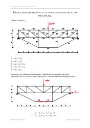
Let us now consider an example <strong>of</strong> <strong>the</strong> assembly process <strong>of</strong> <strong>the</strong> <strong>matrix</strong> K and <strong>the</strong> vector P for a<br />
given plane frame.<br />
M<br />
1 2<br />
1 2<br />
3<br />
q<br />
P<br />
3 4<br />
4 5 y<br />
x
<strong>The</strong> frame consists <strong>of</strong> four beam elements which are interconnected in five nodes. <strong>The</strong> element<br />
<strong>stiffness</strong> matrices and vectors <strong>of</strong> nodal reactions due to <strong>the</strong> span loading are found in <strong>the</strong> local coordinates<br />
for each element<br />
1 2 1 1<br />
1<br />
1<br />
1<br />
x ~<br />
2<br />
y ~ x ~<br />
3<br />
y ~<br />
4<br />
y ~ x ~<br />
y ~ x ~<br />
2<br />
2<br />
are transformed to <strong>the</strong> global co-ordinates<br />
1 2 2 3<br />
1 x<br />
2<br />
y<br />
y<br />
and <strong>the</strong>y can be represented as<br />
x<br />
⎡K11,1<br />
K12,1<br />
⎤ ⎡K11,2<br />
K12,2<br />
⎤ ⎡K11,3<br />
K12,3<br />
⎤ ⎡K11,3<br />
K12,3<br />
⎤<br />
K 1 = ⎢ ⎥ K 2 = ⎢<br />
⎥ K 3 = ⎢<br />
⎥ K 1 = ⎢<br />
⎥<br />
⎣K<br />
21,1 K22,1⎦<br />
⎣K<br />
21,2 K22,2<br />
⎦ ⎣K<br />
21,3 K22,3<br />
⎦ ⎣K<br />
21,3 K22,3<br />
⎦<br />
Note, that <strong>the</strong> local element numbers <strong>of</strong> element nodes can be replaced with <strong>the</strong> global numbers:<br />
Element 1: 1 – 1, 2 – 2, element 2: 1 – 2, 2 – 3, element 3: 1 – 2, 2 – 4, element 4: 1 – 3, 2 – 5.<br />
<strong>The</strong>se relations enable a proper “addressing” <strong>of</strong> <strong>the</strong> subsequent submatrices <strong>of</strong> <strong>the</strong> element<br />
<strong>stiffness</strong> matrices K e in <strong>the</strong> global <strong>stiffness</strong> <strong>matrix</strong> <strong>of</strong> <strong>the</strong> frame K. <strong>The</strong> assembly scheme is<br />
2<br />
4<br />
3<br />
y<br />
x<br />
3<br />
y<br />
4<br />
5<br />
x<br />
K =<br />
K 11,1 K 12,1<br />
K 21,1<br />
K 22,1+K 11,2+<br />
+K 11,3<br />
K 12,2<br />
K 12,3<br />
K 21,2 K 22,2 +K 11,4 K 12,4<br />
K 22,3<br />
K 21,3<br />
K 21,4 K 22,4<br />
Note, that in this scheme each box corresponds to a node and it represents 3×3 elements <strong>of</strong> <strong>the</strong><br />
global <strong>stiffness</strong> <strong>matrix</strong> corresponding to three displacements at <strong>the</strong> given node.<br />
Let us also consider <strong>the</strong> assembly <strong>of</strong> <strong>the</strong> global force vector P.<br />
Out <strong>of</strong> four beams constituting <strong>the</strong> frame only one – No. 4 has a span loading and consequently<br />
<strong>the</strong> non-zero vector <strong>of</strong> reactions due to <strong>the</strong> loading. <strong>The</strong>se vectors for <strong>the</strong> o<strong>the</strong>r beams are zero:<br />
~ ~ ~<br />
R R = R = R = R = R = 0<br />
01 = 02 03 01 02 03<br />
To calculate <strong>the</strong> vector for <strong>the</strong> fourth element <strong>the</strong> loading can be split into uniformly distributed load<br />
acting along <strong>the</strong> beam and transverse to <strong>the</strong> beam<br />
q<br />
q 1 l<br />
q 2<br />
2 l<br />
2<br />
12<br />
q q 2 l<br />
1 = qsinϕcosϕ<br />
q 2 qcos 2 ϕ<br />
l<br />
=<br />
+ 2<br />
l<br />
ϕ<br />
l 2 l<br />
q 1 l<br />
2 2<br />
2 l<br />
2<br />
12
Now <strong>the</strong> vector <strong>of</strong> reactions can be set up<br />
~<br />
R<br />
04<br />
⎡ ~<br />
R<br />
⎢ ~<br />
⎢R<br />
⎢ ~<br />
R<br />
= ⎢ ~<br />
⎢R<br />
⎢ ~<br />
⎢R<br />
⎢ ~<br />
⎣R<br />
01,4<br />
02,4<br />
03,4<br />
04,4<br />
05,4<br />
06,4<br />
and transformed to <strong>the</strong> global set <strong>of</strong> co-ordinates<br />
with <strong>the</strong> transformation <strong>matrix</strong><br />
⎡C<br />
T = ⎢<br />
⎣0<br />
0⎤<br />
⎥<br />
C⎦<br />
R<br />
04<br />
= T<br />
⎡ ql sinϕ<br />
cosϕ<br />
⎤<br />
⎢−<br />
2<br />
⎥<br />
⎢<br />
2 ⎥<br />
⎤ ⎢ ql cos ϕ<br />
−<br />
⎥<br />
⎥ ⎢ 2 ⎥<br />
⎥ ⎢ 2 2<br />
ql cos ϕ ⎥<br />
⎥ ⎢ −<br />
⎥<br />
⎥ = ⎢<br />
⎥<br />
⎥ ⎢ ql sin 12 ϕ cosϕ<br />
−<br />
⎥<br />
⎥ ⎢ 2 ⎥<br />
⎥ ⎢<br />
2<br />
ql cos ϕ ⎥<br />
⎥ ⎢ −<br />
⎥<br />
⎦<br />
⎢ 2 ⎥<br />
2 2<br />
⎢ ql cos ϕ ⎥<br />
⎢<br />
⎣ 12<br />
⎥<br />
⎦<br />
T<br />
4<br />
~<br />
R<br />
04<br />
⎡R<br />
= ⎢<br />
⎣R<br />
01,4<br />
02,4<br />
⎤<br />
⎥<br />
⎦<br />
⎡ cosϕ<br />
⎢<br />
C =<br />
⎢<br />
− sinϕ<br />
⎢⎣<br />
0<br />
sinϕ<br />
cosϕ<br />
<strong>The</strong> nodal external forces P and M are directly substituted into <strong>the</strong> vector <strong>of</strong> loading P, <strong>the</strong> force P<br />
opposite to <strong>the</strong> x axis with <strong>the</strong> negative sign in <strong>the</strong> first <strong>of</strong> three places in <strong>the</strong> box corresponding to<br />
<strong>the</strong> node 3 and <strong>the</strong> clock-wise moment M with <strong>the</strong> positive sign to <strong>the</strong> third place in <strong>the</strong> box<br />
corresponding to <strong>the</strong> node 2.<br />
0<br />
0⎤<br />
⎥<br />
0<br />
⎥<br />
1⎥⎦<br />
P =<br />
–P<br />
0<br />
0<br />
0<br />
0<br />
M<br />
–R 01,4<br />
–R 02,4<br />
<strong>The</strong> global <strong>stiffness</strong> <strong>matrix</strong> K for <strong>the</strong> entire frame has a characteristic band structure. If this band is<br />
narrow a <strong>computer</strong> storage saving is possible. Hence, it is advisable to keep <strong>the</strong> band width as<br />
small as possible. <strong>The</strong> width depends on <strong>the</strong> order <strong>of</strong> node numbering. <strong>The</strong> difference between <strong>the</strong><br />
node numbers for a single element should be kept as small as possible. Let us consider two cases<br />
<strong>of</strong> <strong>the</strong> numbering<br />
1 2 3 4 5<br />
6 7 8 9 10<br />
11 12 13 14 15<br />
1 4 7 10 13<br />
2 5 8 11 14<br />
3 6 9 12 15<br />
In <strong>the</strong> first case <strong>the</strong> maximum difference <strong>of</strong> node numbers for a single element equals to 5 and in<br />
<strong>the</strong> second case – to 3. <strong>The</strong> latter one is <strong>the</strong>refore more efficient because <strong>the</strong> band width in <strong>the</strong><br />
global <strong>stiffness</strong> <strong>matrix</strong> will be smaller.<br />
<strong>The</strong> band width b can be computed as
[ max i − + 1]<br />
b = s ⋅ j<br />
where s is <strong>the</strong> number <strong>of</strong> degrees <strong>of</strong> freedom per node and i and j are <strong>the</strong> node numbers for a<br />
single element. <strong>The</strong> band-structured <strong>matrix</strong> can be stored in <strong>the</strong> <strong>computer</strong> memory as a single<br />
column consisting <strong>of</strong> <strong>the</strong> elements in <strong>the</strong> band read row-wise or as a rectangular <strong>matrix</strong> with <strong>the</strong><br />
dimensions b×n, where n is <strong>the</strong> global number <strong>of</strong> unknown displacements for <strong>the</strong> structure.<br />
<strong>The</strong> assembled global <strong>stiffness</strong> <strong>matrix</strong> K is singular, because it is representing a structure without<br />
any supports, still possessing freedom <strong>of</strong> rigid body rotations. To remove <strong>the</strong> singularity <strong>the</strong><br />
support conditions must be introduced to <strong>the</strong> system <strong>of</strong> equilibrium equations<br />
Kq = P<br />
<strong>The</strong> k-th equation in this set corresponds to <strong>the</strong> condition, that <strong>the</strong> reaction in an additional fictitious<br />
k-th support is zero, as was <strong>the</strong> case in <strong>the</strong> classical <strong>stiffness</strong> <strong>method</strong>. On <strong>the</strong> o<strong>the</strong>r hand, if <strong>the</strong> k-<br />
th support does exist, <strong>the</strong>n <strong>the</strong> corresponding reaction is not zero. Thus, <strong>the</strong> k-th equation is<br />
spurious. Consequently, <strong>the</strong> corresponding displacement q k is zero, hence all <strong>the</strong> elements from<br />
<strong>the</strong> k-th column in <strong>the</strong> <strong>matrix</strong> K multiply <strong>the</strong> zero value and are spurious, too. So, <strong>the</strong> direct <strong>method</strong><br />
<strong>of</strong> inclusion <strong>of</strong> support conditions in <strong>the</strong> equilibrium equations would be to remove <strong>the</strong> rows and<br />
columns from <strong>the</strong> <strong>matrix</strong> K corresponding to <strong>the</strong> real support as well as removing <strong>the</strong><br />
corresponding element from <strong>the</strong> vector P. This <strong>method</strong>, though correct, is not effective numerically,<br />
because it would require a complex process <strong>of</strong> renumbering <strong>of</strong> unknowns.<br />
Instead one <strong>of</strong> several indirect <strong>method</strong>s are used in <strong>computer</strong> practice. <strong>The</strong> first one introduces a<br />
elastic support with an “almost” infinite spring <strong>stiffness</strong>. This leads to a simple addition to <strong>the</strong><br />
element (k,k) in <strong>the</strong> <strong>matrix</strong> K <strong>of</strong> a large number, several orders <strong>of</strong> magnitude larger <strong>the</strong>n <strong>the</strong><br />
maximal element <strong>of</strong> <strong>the</strong> entire <strong>matrix</strong> K.<br />
<strong>The</strong> second <strong>method</strong> modifies <strong>the</strong> k-th equation to a form<br />
1 ⋅ q = 0<br />
k<br />
which automatically yields <strong>the</strong> zero displacement q k in <strong>the</strong> support. This is done by zeroing <strong>the</strong> k-th<br />
element <strong>of</strong> <strong>the</strong> vector P and all <strong>the</strong> elements <strong>of</strong> <strong>the</strong> k-th row <strong>of</strong> <strong>the</strong> <strong>matrix</strong> K except for <strong>the</strong> element<br />
(k,k), which is set to <strong>1.</strong> Additionally, also all <strong>the</strong> elements <strong>of</strong> <strong>the</strong> k-th column <strong>of</strong> <strong>the</strong> <strong>matrix</strong> K are set<br />
to zero to eliminate those that are unnecessary due to <strong>the</strong>ir multiplication by <strong>the</strong> zero displacement<br />
q k .<br />
Existence <strong>of</strong> hinge connections in <strong>the</strong> plane frame requires special care in <strong>the</strong> analysis. For<br />
instance in <strong>the</strong> following example<br />
1 2<br />
1 2<br />
elements 3 and 4 meeting at <strong>the</strong> node 3 have two different angles <strong>of</strong> cross-section rotation <strong>the</strong>re.<br />
So <strong>the</strong> real number <strong>of</strong> unknowns in <strong>the</strong> node 3 is four. If <strong>the</strong> <strong>computer</strong> program allows for such a<br />
situation no problem exists. But if on <strong>the</strong> o<strong>the</strong>r hand <strong>the</strong> number <strong>of</strong> unknowns per node is fixed<br />
than special precautions must be made. If both <strong>the</strong> elements are taken as <strong>the</strong> clamped-hinged<br />
ones with <strong>the</strong> <strong>stiffness</strong> matrices after <strong>the</strong> static condensation, than <strong>the</strong> global <strong>stiffness</strong> <strong>matrix</strong> K will<br />
be singular because <strong>the</strong>re are no non-zero entries to <strong>the</strong> row and column k corresponding <strong>the</strong><br />
rotation(s) in <strong>the</strong> node 3, including 0 on <strong>the</strong> main diagonal. This yields <strong>the</strong> singular equation<br />
0 ⋅ q = 0<br />
One way to overcome this problem is to treat one <strong>of</strong> <strong>the</strong> elements adjacent to <strong>the</strong> hinge, for<br />
instance <strong>the</strong> element 3, as <strong>the</strong> clamped-clamped one with <strong>the</strong> element <strong>matrix</strong> without static<br />
k<br />
3<br />
3 4<br />
4 5
condensation. <strong>The</strong>n, <strong>the</strong> <strong>matrix</strong> K will not be singular and <strong>the</strong> angle <strong>of</strong> rotation at <strong>the</strong> hinge in <strong>the</strong><br />
element 3 will be automatically calculated as one <strong>of</strong> <strong>the</strong> unknowns. <strong>The</strong> element 4 is <strong>the</strong>refore<br />
considered as <strong>the</strong> hinged-clamped one and its <strong>stiffness</strong> <strong>matrix</strong> is obtained from <strong>the</strong> static<br />
condensation.<br />
Influence <strong>of</strong> support displacements can also be included in <strong>the</strong> analysis.<br />
<strong>The</strong>se displacements for an element can be assembled into a vector q ~<br />
∆e<br />
. Like all <strong>the</strong> nodal<br />
displacements, <strong>the</strong>y lead to <strong>the</strong> nodal reactions in elements according to <strong>the</strong> equilibrium equation<br />
for <strong>the</strong> element<br />
~<br />
( q<br />
~<br />
e + q<br />
~<br />
e ) R e<br />
~ ~<br />
R +<br />
e = Ke<br />
∆ 0<br />
<strong>The</strong> influence <strong>of</strong> <strong>the</strong>se displacements can be included in <strong>the</strong> vector <strong>of</strong> reactions due to <strong>the</strong> span<br />
loading<br />
~ ~<br />
( Keq<br />
~<br />
e R e )<br />
~ ~<br />
R<br />
~<br />
+<br />
e = Keqe<br />
+ ∆ 0<br />
Thus, if <strong>the</strong>re is no o<strong>the</strong>r loading <strong>the</strong> support displacements are <strong>the</strong> only factor influencing <strong>the</strong><br />
reactions vector<br />
~ ~<br />
R = K q<br />
~<br />
Let us consider an example<br />
1<br />
0 e<br />
e<br />
∆e<br />
2<br />
2<br />
y ~ x ~<br />
ϕ<br />
γ<br />
∆ x<br />
∆<br />
∆ y<br />
Here only <strong>the</strong> element 2 has “adjacent” support displacements and only its vector <strong>of</strong> reactions will<br />
be non-zero. <strong>The</strong> applied support displacements must be expressed in <strong>the</strong> local co-ordinates <strong>of</strong> <strong>the</strong><br />
element<br />
∆<br />
∆<br />
x<br />
y<br />
= ∆ sinϕ<br />
= ∆ cosϕ<br />
and <strong>the</strong> local vector <strong>of</strong> support displacements for <strong>the</strong> element 2 is<br />
q<br />
~<br />
∆2<br />
⎡ 0 ⎤<br />
⎢ ⎥<br />
⎢<br />
0<br />
⎥<br />
⎢ 0 ⎥<br />
= ⎢ ⎥<br />
⎢∆<br />
x ⎥<br />
⎢∆<br />
⎥<br />
y<br />
⎢ ⎥<br />
⎢⎣<br />
− γ ⎥⎦<br />
Note, that <strong>the</strong> displacements must be substituted with appropriate sign according to <strong>the</strong>ir<br />
orientation with respect to <strong>the</strong> local axes. <strong>The</strong>refore, <strong>the</strong> anti-clockwise rotation is taken as<br />
negative.<br />
Having this vector <strong>of</strong> displacements <strong>the</strong> corresponding vector <strong>of</strong> reactions can be calculated,<br />
transformed to <strong>the</strong> global co-ordinates and used in <strong>the</strong> assembly process <strong>of</strong> <strong>the</strong> vector <strong>of</strong> nodal<br />
forces P.
Let us now set <strong>the</strong> entire algorithm <strong>of</strong> <strong>the</strong> <strong>matrix</strong> <strong>version</strong> <strong>of</strong> <strong>the</strong> <strong>stiffness</strong> <strong>method</strong> for <strong>the</strong> plane<br />
frames.<br />
<strong>1.</strong> Assume <strong>the</strong> global co-ordinate system. Number <strong>the</strong> nodes and element. Select <strong>the</strong> local<br />
systems <strong>of</strong> co-ordinates. Attach <strong>the</strong> internal hinged connections to <strong>the</strong> elements leaving one<br />
element at a hinge as clamped-clamped.<br />
2. Calculate local <strong>stiffness</strong> matrices K ~ e for <strong>the</strong> elements with <strong>the</strong> static condensation for <strong>the</strong><br />
hinged-clamped ones. Transform <strong>the</strong> local matrices to <strong>the</strong> global co-ordinates to get K e<br />
T ~<br />
K = T K T<br />
e<br />
3. Assemble <strong>the</strong> global <strong>stiffness</strong> <strong>matrix</strong> K for <strong>the</strong> entire system from all <strong>the</strong> element matrices K e<br />
expressed in global so-ordinates.<br />
~<br />
4. Calculate <strong>the</strong> vectors <strong>of</strong> reactions R 0e<br />
due to <strong>the</strong> span loading: forces on <strong>the</strong> beams, uniform<br />
and non-uniform heating, support displacements. Transform <strong>the</strong>se vectors to <strong>the</strong> global coordinates<br />
to get R 0e .<br />
e<br />
e<br />
~<br />
e<br />
T<br />
0e Te<br />
R0e<br />
R =<br />
5. Assemble <strong>the</strong> vector <strong>of</strong> nodal forces P for <strong>the</strong> entire system from all <strong>the</strong> element vectors R 0e<br />
taken with <strong>the</strong> negative sign and all <strong>the</strong> external nodal loading.<br />
6. Include <strong>the</strong> supports in K and P. For <strong>the</strong> rigid supports set to zero all <strong>the</strong> corresponding<br />
elements in P and all <strong>the</strong> elements in <strong>the</strong> corresponding rows and columns <strong>of</strong> K except for <strong>the</strong><br />
main diagonal term to be set to <strong>1.</strong> For <strong>the</strong> flexible supports add <strong>the</strong> spring <strong>stiffness</strong> to <strong>the</strong><br />
corresponding main diagonal term in K.<br />
7. Solve <strong>the</strong> global set <strong>of</strong> equilibrium equations<br />
Kq = P<br />
to get <strong>the</strong> nodal displacements in global co-ordinates.<br />
8. Select <strong>the</strong> displacements for <strong>the</strong> separate elements and form <strong>the</strong> appropriate vectors q e .<br />
Transform <strong>the</strong>se vectors to <strong>the</strong> local co-ordinates to get q ~<br />
e<br />
q<br />
~<br />
= T q<br />
e<br />
9. Compute <strong>the</strong> reactions at <strong>the</strong> element ends from <strong>the</strong> equilibrium conditions for <strong>the</strong> separate<br />
elements<br />
e<br />
e<br />
~ ~ ~ ~<br />
R = K q + R<br />
e e e 0e<br />
<strong>The</strong>se reactions correspond to <strong>the</strong> values <strong>of</strong> internal forces at <strong>the</strong> element ends<br />
~<br />
R<br />
e<br />
⎡ ~<br />
R<br />
⎢ ~<br />
⎢R<br />
⎢ ~<br />
R<br />
= ⎢ ~<br />
⎢R<br />
⎢ ~<br />
⎢<br />
R<br />
~<br />
⎢⎣<br />
R<br />
1<br />
2<br />
3<br />
4<br />
5<br />
6<br />
⎤ ⎡−<br />
N<br />
⎥ ⎢<br />
⎥ ⎢<br />
−T<br />
⎥ ⎢ Mik<br />
⎥ = ⎢<br />
⎥ ⎢ Nki<br />
⎥ ⎢ Tki<br />
⎥ ⎢<br />
⎥⎦<br />
⎢⎣<br />
Mki<br />
ik<br />
ik<br />
⎤<br />
⎥<br />
⎥<br />
⎥<br />
⎥<br />
⎥<br />
⎥<br />
⎥<br />
⎥⎦<br />
At <strong>the</strong> end let us summarise some “tricks” related to <strong>the</strong> <strong>matrix</strong> <strong>version</strong> <strong>of</strong> <strong>the</strong> <strong>stiffness</strong> <strong>method</strong>.<br />
<strong>1.</strong> Flexible support as an additional element<br />
k EA<br />
= k , EI = 0<br />
l
2. A truss can be solved using <strong>the</strong> beam elements if one element <strong>of</strong> those meeting at a node is<br />
treated as clamped.<br />
For <strong>the</strong> hinged-hinged elements <strong>the</strong> static condensation <strong>of</strong> <strong>the</strong> <strong>matrix</strong> for clamped-hinged element<br />
can be carried out to eliminate <strong>the</strong> second rotation.<br />
3. Curved beams can be analysed in an approximate way by modelling <strong>the</strong> curve as an assembly<br />
<strong>of</strong> a sufficiently large number <strong>of</strong> straight-line beams<br />
4. Similarly, tapered elements can be modelled as assemblies <strong>of</strong> piece-wise constant cross-section<br />
elements.<br />
5. Calculation <strong>of</strong> displacement at an arbitrary point <strong>of</strong> an element<br />
A<br />
v A<br />
q<br />
q<br />
~<br />
3<br />
q<br />
~<br />
q<br />
~<br />
1<br />
2<br />
v A0<br />
A<br />
q<br />
~<br />
5<br />
q<br />
~<br />
6<br />
q<br />
~<br />
4<br />
<strong>The</strong> arbitrary displacement can be calculated using <strong>the</strong> superposition rule applied to <strong>the</strong> influences<br />
<strong>of</strong> <strong>the</strong> support (nodal) displacements and <strong>the</strong> span loading. Hence, we have<br />
v<br />
A<br />
= v<br />
A0<br />
<strong>The</strong> displacements along <strong>the</strong> element due to <strong>the</strong> nodal displacements are calculated using so<br />
called shape functions. In <strong>the</strong> case <strong>of</strong> <strong>the</strong> beam element axial nodal displacements do not cause<br />
transverse displacements in <strong>the</strong> beam. So <strong>the</strong> non-zero shape functions are due to <strong>the</strong><br />
displacements 2, 3, 5 and 6. <strong>The</strong>y have <strong>the</strong> form<br />
q<br />
~<br />
v A6<br />
q<br />
~<br />
6<br />
3<br />
A<br />
A<br />
A<br />
q<br />
~<br />
2<br />
v A2<br />
v A3<br />
+<br />
6<br />
∑<br />
i = 1<br />
v<br />
~<br />
Ai q i<br />
v A5 q<br />
~<br />
5<br />
A<br />
and <strong>the</strong> exact ma<strong>the</strong>matical expressions will be derived in <strong>the</strong> following section on <strong>matrix</strong> analysis<br />
<strong>of</strong> stability <strong>of</strong> frames.
6. Calculation <strong>of</strong> envelopes <strong>of</strong> static and kinematic quantities under a set <strong>of</strong> moving loads.<br />
For instance let us consider <strong>the</strong> envelope <strong>of</strong> bending moments in <strong>the</strong> beam presented in <strong>the</strong> figure<br />
q P 1 P 2<br />
<strong>The</strong> classical approach involves calculation <strong>of</strong> influence lines. <strong>The</strong>y are found for <strong>the</strong> moments at<br />
several number <strong>of</strong> points along <strong>the</strong> beam. Each influence line is loaded by <strong>the</strong> load set in <strong>the</strong> way<br />
leading to <strong>the</strong> extreme output moments (positive and negative) calculated from <strong>the</strong> superposition<br />
rule.<br />
0 1 2 etc.<br />
M 0 (x)<br />
q P 1 P 2<br />
M 1 (x)<br />
M 2 (x)<br />
etc.<br />
S<br />
η 1<br />
η 2<br />
M<br />
M<br />
2max<br />
2min<br />
= max<br />
= min<br />
( qS + P1<br />
η1<br />
+ P2η<br />
2 )<br />
( qS + Pη<br />
+ P η )<br />
<strong>The</strong>se maximum values are <strong>the</strong>n put toge<strong>the</strong>r to yield <strong>the</strong> envelope.<br />
1<br />
1<br />
2<br />
2<br />
0 1 2 etc.<br />
M 2min<br />
M 2max<br />
etc.<br />
7. Solving a set <strong>of</strong> algebraic equations<br />
AX = B<br />
For a simple calculation <strong>of</strong> unknowns X <strong>the</strong> main <strong>matrix</strong> <strong>of</strong> coefficients A can be decomposed into<br />
a product <strong>of</strong> two triangular matrices<br />
A = A 1 A 2<br />
=<br />
0<br />
·<br />
0<br />
to get<br />
<strong>The</strong> product<br />
A A X = B<br />
1<br />
2<br />
A 2 X =<br />
Z
gives an auxiliary vector and <strong>the</strong> original set <strong>of</strong> equations is represented as a combination <strong>of</strong> two<br />
sets <strong>of</strong> equations<br />
A Z = B<br />
1<br />
A X = Z<br />
2<br />
Each <strong>of</strong> <strong>the</strong>se sets is characterised be a triangular coefficient <strong>matrix</strong> and can be easily solved<br />
equation after equation by a <strong>method</strong> <strong>of</strong> back substitution.<br />
<strong>The</strong> decomposition into two triangular matrices can be done be several <strong>method</strong>s, e.g. <strong>the</strong> classical<br />
Gauss elimination <strong>method</strong> or <strong>the</strong> Choleski <strong>method</strong>. In <strong>the</strong> latter one<br />
so we have<br />
T<br />
2<br />
A = A = S<br />
1<br />
T<br />
S SX = B<br />
and <strong>the</strong> process <strong>of</strong> back substitution is even simpler because just one triangular <strong>matrix</strong> S must be<br />
stored in <strong>the</strong> <strong>computer</strong> memory.<br />
Example<br />
Let us find <strong>the</strong> distribution <strong>of</strong> internal forces in <strong>the</strong> following frame using <strong>the</strong> <strong>matrix</strong> <strong>version</strong> <strong>of</strong> <strong>the</strong><br />
<strong>stiffness</strong> <strong>method</strong>.<br />
10<br />
20kN/m<br />
Data:<br />
8<br />
E = 205 GPa<br />
7<br />
9 2<br />
x<br />
20kN 2 β k<br />
k = 57195 kN/m<br />
4<br />
y<br />
β = arctan2/5 = 2<strong>1.</strong>801°<br />
6 5<br />
Element 1:<br />
A = 27.9cm 2<br />
1<br />
4<br />
I = 1450cm 4<br />
3<br />
l = 4m<br />
Element 2:<br />
1<br />
5<br />
[m]<br />
A = 46.1 cm 2<br />
2<br />
I = 4250 cm 4<br />
l = 5.3852 m<br />
In <strong>the</strong> solution we will use <strong>the</strong> <strong>method</strong> without constant number <strong>of</strong> unknowns in <strong>the</strong> node. <strong>The</strong><br />
hinge connecting both elements is <strong>the</strong>refore <strong>the</strong> node with four unknown displacements including<br />
two separate angles <strong>of</strong> rotation, one for each element.<br />
Both elements will be considered as clamped-hinged ones and <strong>the</strong> corresponding <strong>stiffness</strong><br />
matrices and vectors <strong>of</strong> reactions will be found for such elements. In <strong>the</strong> following figures<br />
displacement directions for both elements are shown in local and global co-ordinates and <strong>the</strong> angle<br />
α for <strong>the</strong> transformation is found.<br />
4 x ~ 1<br />
6<br />
5<br />
5<br />
6<br />
4<br />
x ~<br />
α = 270°<br />
3<br />
3<br />
y<br />
2<br />
α x<br />
1<br />
1<br />
2<br />
1<br />
Local co-ordinates Global co-ordinates Transformation
1<br />
6<br />
α = 360°–β = 338.199°<br />
4 x ~ 6<br />
4<br />
3<br />
2 5<br />
3<br />
x ~ 2 5<br />
β<br />
2<br />
1<br />
α x<br />
y ~ 2<br />
Local co-ordinates Global co-ordinates Transformation<br />
Now we can associate <strong>the</strong> numbers <strong>of</strong> nodal displacements in <strong>the</strong> elements expressed in global<br />
co-ordinates (from 1 to 6 for each element) with <strong>the</strong> numbers <strong>of</strong> nodal displacements in <strong>the</strong> global<br />
numbering (from 1 to 10 in <strong>the</strong> considered example). Thus <strong>the</strong> allocation table is created<br />
Element<br />
Element directions<br />
number 1 2 3 4 5 6<br />
1 1 2 3 4 5 6<br />
2 4 5 7 8 9 10<br />
<strong>The</strong>se allocations indicate, where <strong>the</strong> subsequent values from <strong>the</strong> element matrices and vectors in<br />
global co-ordinates enter <strong>the</strong> global matrices and vectors for <strong>the</strong> entire structure. For instance: <strong>the</strong><br />
value k 52,2 from <strong>the</strong> <strong>stiffness</strong> <strong>matrix</strong> K 2 is added to <strong>the</strong> element k 59 in <strong>the</strong> global <strong>matrix</strong> K, <strong>the</strong> value<br />
R 06,2 from <strong>the</strong> vector <strong>of</strong> reactions R 02 is subtracted from <strong>the</strong> element P 10 in <strong>the</strong> global vector P.<br />
Now let us find <strong>the</strong> reactions vectors due to span loading. In this case only element 2 is loaded and<br />
<strong>the</strong> loading is split into two components:<br />
q<br />
q<br />
x<br />
y<br />
= 6sin β cos β = 2.0689 kN/m<br />
2<br />
= 6cos β = 5.1725 kN/m<br />
6<br />
6<br />
3<br />
q x<br />
5<br />
4<br />
3<br />
q y<br />
5<br />
4<br />
1<br />
2<br />
1<br />
2<br />
For <strong>the</strong> clamped-hinged element <strong>the</strong> vector <strong>of</strong> reactions is<br />
~<br />
R<br />
02<br />
⎡ ~<br />
R<br />
⎢ ~<br />
⎢R<br />
⎢ ~<br />
= ⎢<br />
R<br />
~<br />
⎢R<br />
⎢ ~<br />
⎢R<br />
⎢ ~<br />
⎣R<br />
01,2<br />
02,2<br />
03,2<br />
04,2<br />
05,2<br />
06,2<br />
⎡ qxl<br />
⎤<br />
⎢ ⎥<br />
⎤ ⎢<br />
3 2<br />
q<br />
⎥<br />
⎢<br />
yl<br />
⎡ 5.5708 ⎤<br />
⎥ − ⎥<br />
⎢ ⎥<br />
⎥ ⎢ ⎥<br />
⎢<br />
−10.446<br />
⎥<br />
⎥<br />
⎥ ⎢ 0 8<br />
⎥<br />
⎢ ⎥<br />
⎥ = ⎢ q<br />
0<br />
xl<br />
=<br />
⎢ ⎥<br />
⎢ ⎥<br />
⎥<br />
⎢ ⎥<br />
⎢ 5.5708 ⎥<br />
⎥<br />
⎢<br />
5 2 q<br />
⎥<br />
⎢−<br />
⎥<br />
⎥<br />
yl<br />
17.409<br />
−<br />
⎢ ⎥<br />
⎢ ⎥<br />
⎥ 8<br />
⎦<br />
⎢⎣<br />
18.750 ⎥<br />
⎢ 2 ⎥<br />
⎦<br />
q l<br />
⎢<br />
y<br />
⎥<br />
⎢⎣<br />
8 ⎥⎦<br />
<strong>The</strong> element <strong>stiffness</strong> matrices in <strong>the</strong> local co-ordinates are
⎥<br />
⎥<br />
⎥<br />
⎥<br />
⎥<br />
⎥<br />
⎥<br />
⎥<br />
⎦<br />
⎤<br />
⎢<br />
⎢<br />
⎢<br />
⎢<br />
⎢<br />
⎢<br />
⎢<br />
⎢<br />
⎣<br />
⎡<br />
−<br />
−<br />
−<br />
−<br />
−<br />
−<br />
=<br />
⎥<br />
⎥<br />
⎥<br />
⎥<br />
⎥<br />
⎥<br />
⎥<br />
⎥<br />
⎥<br />
⎥<br />
⎥<br />
⎥<br />
⎦<br />
⎤<br />
⎢<br />
⎢<br />
⎢<br />
⎢<br />
⎢<br />
⎢<br />
⎢<br />
⎢<br />
⎢<br />
⎢<br />
⎢<br />
⎢<br />
⎣<br />
⎡<br />
−<br />
−<br />
−<br />
−<br />
−<br />
−<br />
=<br />
0<br />
0<br />
0<br />
0<br />
0<br />
0<br />
0<br />
139.3<br />
0<br />
557.3<br />
139.3<br />
0<br />
0<br />
0<br />
143000<br />
0<br />
0<br />
14300<br />
0<br />
557.3<br />
0<br />
2229<br />
557.3<br />
0<br />
0<br />
139.3<br />
0<br />
557.3<br />
139.3<br />
0<br />
0<br />
0<br />
143000<br />
0<br />
0<br />
143000<br />
0<br />
0<br />
0<br />
0<br />
0<br />
0<br />
0<br />
3<br />
0<br />
6<br />
3<br />
0<br />
0<br />
0<br />
0<br />
0<br />
0<br />
3<br />
0<br />
3<br />
3<br />
0<br />
0<br />
3<br />
0<br />
3<br />
3<br />
0<br />
0<br />
0<br />
0<br />
0<br />
~<br />
3<br />
2<br />
3<br />
2<br />
2<br />
3<br />
2<br />
3<br />
1<br />
l<br />
EI<br />
l<br />
EI<br />
l<br />
EI<br />
l<br />
EA<br />
l<br />
EA<br />
l<br />
EI<br />
l<br />
EI<br />
l<br />
EI<br />
l<br />
EI<br />
l<br />
EI<br />
l<br />
EI<br />
l<br />
EA<br />
l<br />
EA<br />
K<br />
⎥<br />
⎥<br />
⎥<br />
⎥<br />
⎥<br />
⎥<br />
⎥<br />
⎥<br />
⎦<br />
⎤<br />
⎢<br />
⎢<br />
⎢<br />
⎢<br />
⎢<br />
⎢<br />
⎢<br />
⎢<br />
⎣<br />
⎡<br />
−<br />
−<br />
−<br />
−<br />
−<br />
−<br />
=<br />
⎥<br />
⎥<br />
⎥<br />
⎥<br />
⎥<br />
⎥<br />
⎥<br />
⎥<br />
⎥<br />
⎥<br />
⎥<br />
⎥<br />
⎦<br />
⎤<br />
⎢<br />
⎢<br />
⎢<br />
⎢<br />
⎢<br />
⎢<br />
⎢<br />
⎢<br />
⎢<br />
⎢<br />
⎢<br />
⎢<br />
⎣<br />
⎡<br />
−<br />
−<br />
−<br />
−<br />
−<br />
−<br />
=<br />
4854<br />
90<strong>1.</strong>3<br />
0<br />
0<br />
90<strong>1.</strong>3<br />
0<br />
90<strong>1.</strong>3<br />
167.4<br />
0<br />
0<br />
167.4<br />
0<br />
0<br />
0<br />
175500<br />
0<br />
0<br />
175500<br />
0<br />
0<br />
0<br />
0<br />
0<br />
0<br />
90<strong>1.</strong>3<br />
167.4<br />
0<br />
0<br />
167.4<br />
0<br />
0<br />
0<br />
175500<br />
0<br />
0<br />
175500<br />
3<br />
3<br />
0<br />
0<br />
3<br />
0<br />
3<br />
3<br />
0<br />
0<br />
3<br />
0<br />
0<br />
0<br />
0<br />
0<br />
0<br />
0<br />
0<br />
0<br />
0<br />
0<br />
3<br />
3<br />
0<br />
0<br />
3<br />
0<br />
0<br />
0<br />
0<br />
0<br />
~<br />
2<br />
2<br />
2<br />
3<br />
3<br />
2<br />
3<br />
3<br />
2<br />
l<br />
EI<br />
l<br />
EI<br />
l<br />
EI<br />
l<br />
EI<br />
l<br />
EI<br />
l<br />
EI<br />
l<br />
EA<br />
l<br />
EA<br />
l<br />
EI<br />
l<br />
EI<br />
l<br />
EI<br />
l<br />
EA<br />
l<br />
EA<br />
K<br />
<strong>The</strong> transformation matrices are<br />
⎥<br />
⎦<br />
⎤<br />
⎢<br />
⎣<br />
⎡<br />
=<br />
C<br />
0<br />
0<br />
C<br />
T e<br />
⎥<br />
⎥<br />
⎥<br />
⎦<br />
⎤<br />
⎢<br />
⎢<br />
⎢<br />
⎣<br />
⎡<br />
−<br />
=<br />
1<br />
0<br />
0<br />
0<br />
cos<br />
sin<br />
0<br />
sin<br />
cos<br />
α<br />
α<br />
α<br />
α<br />
C<br />
⎥<br />
⎥<br />
⎥<br />
⎥<br />
⎥<br />
⎥<br />
⎥<br />
⎥<br />
⎦<br />
⎤<br />
⎢<br />
⎢<br />
⎢<br />
⎢<br />
⎢<br />
⎢<br />
⎢<br />
⎢<br />
⎣<br />
⎡<br />
−<br />
−<br />
=<br />
1<br />
0<br />
0<br />
0<br />
0<br />
0<br />
0<br />
0<br />
1<br />
0<br />
0<br />
0<br />
0<br />
1<br />
0<br />
0<br />
0<br />
0<br />
0<br />
0<br />
0<br />
1<br />
0<br />
0<br />
0<br />
0<br />
0<br />
0<br />
0<br />
1<br />
0<br />
0<br />
0<br />
0<br />
1<br />
0<br />
1<br />
T<br />
⎥<br />
⎥<br />
⎥<br />
⎥<br />
⎥<br />
⎥<br />
⎥<br />
⎥<br />
⎦<br />
⎤<br />
⎢<br />
⎢<br />
⎢<br />
⎢<br />
⎢<br />
⎢<br />
⎢<br />
⎢<br />
⎣<br />
⎡<br />
−<br />
−<br />
=<br />
1<br />
0<br />
0<br />
0<br />
0<br />
0<br />
0<br />
0.9285<br />
0.3714<br />
0<br />
0<br />
0<br />
0<br />
0.3714<br />
0.9285<br />
0<br />
0<br />
0<br />
0<br />
0<br />
0<br />
1<br />
0<br />
0<br />
0<br />
0<br />
0<br />
0<br />
0.9285<br />
0.3714<br />
0<br />
0<br />
0<br />
0<br />
0.3714<br />
0.9285<br />
2<br />
T<br />
Now <strong>the</strong> transformation <strong>of</strong> local matrices and vectors to <strong>the</strong> global co-ordinates can be done.<br />
⎥<br />
⎥<br />
⎥<br />
⎥<br />
⎥<br />
⎥<br />
⎥<br />
⎥<br />
⎦<br />
⎤<br />
⎢<br />
⎢<br />
⎢<br />
⎢<br />
⎢<br />
⎢<br />
⎢<br />
⎢<br />
⎣<br />
⎡<br />
−<br />
−<br />
−<br />
=<br />
=<br />
18.750<br />
18.233<br />
<strong>1.</strong>2929<br />
0<br />
1<strong>1.</strong>768<br />
<strong>1.</strong>2929<br />
~<br />
02<br />
2<br />
02 R<br />
T<br />
R<br />
T<br />
⎥<br />
⎥<br />
⎥<br />
⎥<br />
⎥<br />
⎥<br />
⎥<br />
⎥<br />
⎦<br />
⎤<br />
⎢<br />
⎢<br />
⎢<br />
⎢<br />
⎢<br />
⎢<br />
⎢<br />
⎢<br />
⎣<br />
⎡<br />
−<br />
−<br />
−<br />
−<br />
−<br />
−<br />
−<br />
−<br />
=<br />
=<br />
0<br />
0<br />
0<br />
0<br />
0<br />
0<br />
0<br />
24350<br />
60460<br />
0<br />
24350<br />
60460<br />
0<br />
60460<br />
151300<br />
0<br />
60460<br />
151300<br />
0<br />
0<br />
0<br />
2229<br />
0<br />
557.3<br />
0<br />
24350<br />
60460<br />
0<br />
143000<br />
0<br />
0<br />
60460<br />
151300<br />
557.3<br />
0<br />
139.3<br />
~<br />
~<br />
1<br />
1<br />
1<br />
1 T<br />
K<br />
T<br />
K<br />
T
~ T ~<br />
K2 = T2<br />
K2T<br />
2<br />
⎡ 151300<br />
⎢<br />
⎢<br />
− 60460<br />
⎢ 0<br />
= ⎢<br />
⎢−151300<br />
⎢ − 60460<br />
⎢<br />
⎢⎣<br />
334.7<br />
− 60460<br />
24350<br />
0<br />
60460<br />
− 24350<br />
90<strong>1.</strong>3<br />
0<br />
0<br />
0<br />
0<br />
0<br />
0<br />
−151300<br />
60460<br />
0<br />
151300<br />
− 60460<br />
− 334.7<br />
− 60460<br />
− 24350<br />
0<br />
− 60460<br />
24350<br />
− 836.8<br />
334.7 ⎤<br />
⎥<br />
90<strong>1.</strong>3<br />
⎥<br />
0 ⎥<br />
⎥<br />
− 334.7⎥<br />
− 836.8⎥<br />
⎥<br />
4854 ⎥⎦<br />
Following <strong>the</strong> relations in <strong>the</strong> allocation table <strong>the</strong> following scheme <strong>of</strong> assembly <strong>of</strong> <strong>the</strong> global<br />
<strong>stiffness</strong> <strong>matrix</strong> and <strong>the</strong> global force vector is created.<br />
k 11,1 k 12,1 k 13,1 k 14,1 k 15,1 k 16,1 –R 01,1<br />
k 22,1 k 23,1 k 24,1 k 25,1 k 26,1 –R 02,1<br />
k 33,1 k 34,1 k 35,1 k 36,1 –R 03,1<br />
k 44,1 k 45,1 k 46,1 –R 04,1<br />
k 55,1 k 56,1 –R 05,1<br />
k 66,1 –R 06,1<br />
s y m m e t r y<br />
k 11,2 k 12,2 k 13,2 k 14,2 k 15,2 k 16,2 –R 01,2<br />
k 22,2 k 23,2 k 24,2 k 25,2 k 26,2 –R 02,2<br />
k 33,2 k 34,2 k 35,2 k 36,2 –R 03,2<br />
k 44,2 k 45,2 k 46,2 –R 04,2<br />
s y m m e t r y k 55,2 k 56,2 –R 05,2<br />
k 66,2 –R 06,2<br />
Both <strong>the</strong> elements contribute simultaneously to <strong>the</strong> values k 44 , k 45 , k 54 and k 55 in <strong>the</strong> <strong>stiffness</strong> <strong>matrix</strong><br />
K. <strong>The</strong> appropriate values from <strong>the</strong> element <strong>stiffness</strong> matrices are added in <strong>the</strong>se windows. Due to<br />
<strong>the</strong> elastic support in <strong>the</strong> direction <strong>of</strong> <strong>the</strong> displacement 9 requires an addition <strong>of</strong> <strong>the</strong> spring <strong>stiffness</strong><br />
k in <strong>the</strong> value k 99 <strong>of</strong> <strong>the</strong> global <strong>stiffness</strong> <strong>matrix</strong> K. <strong>The</strong> nodal force 20kN acting along <strong>the</strong> direction 4<br />
in its positive orientation must be added to <strong>the</strong> element P 4 <strong>of</strong> <strong>the</strong> vector P.<br />
Thus <strong>the</strong> global <strong>matrix</strong> K and <strong>the</strong> vector P are formed.<br />
139.3 0 557.3 –139.3 0 0 0 0 0 0 0<br />
143000 0 0 –143000 0 0 0 0 0 0<br />
2229 –557.3 0 0 0 0 0 0 0<br />
151439 –60460 0 0 –151300 60460 334.7 18.707<br />
167350 0 0 60460 –24350 836.8 1<strong>1.</strong>768<br />
0 0 0 0 0 0<br />
0 0 0 0 0<br />
81545 –60460 –334.7 <strong>1.</strong>2931<br />
s y m m e t r y 24350 –836.8 18.233<br />
4854 –18.750
Now <strong>the</strong> support conditions must be included. In <strong>the</strong> analyzed frame <strong>the</strong> following support<br />
displacements are zero:<br />
q<br />
= q q q q<br />
1 2 = 3 = 8 = 10 =<br />
Thus, <strong>the</strong> 1 st , 2 nd , 3 rd , 8 th and 10 th elements in <strong>the</strong> vector P and <strong>the</strong> elements in <strong>the</strong> 1 st , 2 nd , 3 rd , 8 th<br />
and 10 th rows and columns <strong>of</strong> K must be set to zero except for <strong>the</strong> elements at <strong>the</strong> diagonal <strong>of</strong> K,<br />
which are set to <strong>1.</strong><br />
<strong>The</strong> rotations at <strong>the</strong> hinge q 6 and q 7 are not zero but were eliminated on <strong>the</strong> element level by <strong>the</strong><br />
static condensation. Thus, <strong>the</strong>y also must be eliminated from <strong>the</strong> global set <strong>of</strong> equations. This can<br />
be done by setting <strong>the</strong> elements k 66 and k 77 at <strong>the</strong> diagonal <strong>of</strong> K to <strong>1.</strong> Thus <strong>the</strong> rotations will be kept<br />
in <strong>the</strong> vector <strong>of</strong> unknowns and <strong>the</strong>ir values will be calculated as 0. Despite <strong>the</strong> fact, that <strong>the</strong>se<br />
values are not true, <strong>the</strong>y will not be used in fur<strong>the</strong>r calculations, because <strong>the</strong>y were indeed<br />
eliminated. <strong>The</strong>y will be denoted with asterisks.<br />
Thus we get <strong>the</strong> final form <strong>of</strong> <strong>the</strong> global set <strong>of</strong> equilibrium equations<br />
0<br />
1 0 0 0 0 0 0 0 0 0 0<br />
1 0 0 0 0 0 0 0 0 0<br />
1 0 0 0 0 0 0 0 0<br />
151439 –60460 0 0 0 60460 0 18.707<br />
167350 0 0 0 –24350 0 1<strong>1.</strong>768<br />
1 0 0 0 0 0<br />
1 0 0 0 0<br />
1 0 0 0<br />
s y m m e t r y 24350 0 18.233<br />
1 0<br />
Solving <strong>of</strong> <strong>the</strong> equations<br />
Kq = P<br />
Yields <strong>the</strong> following vector <strong>of</strong> global displacements<br />
⎡ 0 ⎤<br />
⎢ ⎥<br />
⎢<br />
0<br />
⎥<br />
⎢ 0 ⎥<br />
⎢ ⎥<br />
⎢0.0001022⎥<br />
⎢0.0001346⎥<br />
q = ⎢ ⎥<br />
⎢ 0 * ⎥<br />
⎢ 0 * ⎥<br />
⎢ ⎥<br />
⎢ 0 ⎥<br />
⎢ ⎥<br />
⎢<br />
0.0001880<br />
⎥<br />
⎢⎣<br />
0 ⎥⎦<br />
Following <strong>the</strong> relations in <strong>the</strong> allocation table <strong>the</strong> appropriate displacements can be attributed to <strong>the</strong><br />
elements and <strong>the</strong> element vectors <strong>of</strong> displacements in global co-ordinates can be formed.
q<br />
1<br />
⎡q<br />
⎢<br />
⎢<br />
q<br />
⎢q<br />
= ⎢<br />
⎢q<br />
⎢q<br />
⎢<br />
⎢⎣<br />
q<br />
1<br />
2<br />
3<br />
4<br />
5<br />
6<br />
⎤ ⎡ 0 ⎤<br />
⎥ ⎢ ⎥<br />
⎥ ⎢<br />
0<br />
⎥<br />
⎥ ⎢ 0 ⎥<br />
⎥ = ⎢ ⎥<br />
⎥ ⎢0.0001022⎥<br />
⎥ ⎢0.0001346⎥<br />
⎥ ⎢ ⎥<br />
⎥⎦<br />
⎢⎣<br />
0 * ⎥⎦<br />
q<br />
2<br />
⎡q<br />
⎢<br />
⎢<br />
q<br />
⎢q<br />
= ⎢<br />
⎢q<br />
⎢q<br />
⎢<br />
⎢⎣<br />
q<br />
<strong>The</strong>se vectors can be transformed to local co-ordinates<br />
q<br />
~<br />
1 = T1q<br />
1<br />
q<br />
~<br />
2 = T1q<br />
2<br />
to get<br />
⎡ 0 ⎤<br />
⎢<br />
⎥<br />
⎢<br />
0<br />
⎥<br />
⎢ 0 ⎥<br />
q<br />
~<br />
1 = ⎢<br />
⎥<br />
⎢−<br />
0.0001346⎥<br />
⎢ 0.0001022 ⎥<br />
⎢<br />
⎥<br />
⎢⎣<br />
0 * ⎥⎦<br />
1<br />
2<br />
3<br />
4<br />
5<br />
6<br />
⎤ ⎡0.0001022⎤<br />
⎥ ⎢ ⎥<br />
⎥ ⎢<br />
0.0001346<br />
⎥<br />
⎥ ⎢ 0 * ⎥<br />
⎥ = ⎢ ⎥<br />
⎥ ⎢ 0 ⎥<br />
⎥ ⎢0.0001880⎥<br />
⎥ ⎢ ⎥<br />
⎥⎦<br />
⎢⎣<br />
0 * ⎥⎦<br />
⎡ 0.0000449 ⎤<br />
⎢<br />
⎥<br />
⎢<br />
0.0001629<br />
⎥<br />
⎢ 0 * ⎥<br />
q<br />
~<br />
2 = ⎢<br />
⎥<br />
⎢−<br />
0.0000698⎥<br />
⎢ 0.0001746 ⎥<br />
⎢<br />
⎥<br />
⎢⎣<br />
0 ⎥⎦<br />
With <strong>the</strong>se vectors <strong>the</strong> final values <strong>of</strong> nodal reactions can be found<br />
~ ~ ~ ~<br />
R +<br />
1 = K1q1<br />
R01<br />
R 2 = K2q2<br />
+ R02<br />
⎡ 19.248 ⎤<br />
⎢ ⎥<br />
⎢<br />
− 0.014<br />
⎥<br />
~ ⎢ − 0.057 ⎥<br />
R 1 = ⎢ ⎥<br />
⎢−19.248⎥<br />
⎢ 0.014 ⎥<br />
⎢ ⎥<br />
⎢⎣<br />
0 ⎥⎦<br />
~<br />
~<br />
~<br />
~<br />
⎡ 25.701 ⎤<br />
⎢ ⎥<br />
⎢<br />
−10.448<br />
⎥<br />
~ ⎢ 0 ⎥<br />
R 2 = ⎢ ⎥<br />
⎢−14.559⎥<br />
⎢−17.407⎥<br />
⎢ ⎥<br />
⎢⎣<br />
18.740 ⎥⎦<br />
Note, that <strong>the</strong> values <strong>of</strong> rotations at <strong>the</strong> hinge denoted by 0* are indeed not necessary, because<br />
<strong>the</strong>y are multiplied by zeros in 6 th or 3 rd column in <strong>the</strong> <strong>stiffness</strong> matrices for <strong>the</strong> element 1 and 2,<br />
respectively.<br />
<strong>The</strong>se reactions can be finally used to find <strong>the</strong> distributions <strong>of</strong> <strong>the</strong> internal forces<br />
–25.7<br />
–<br />
–14.6<br />
10.4<br />
+ –<br />
18.74<br />
N [kN]<br />
– –19.2<br />
+ 0.014<br />
–17.4<br />
T [kN]<br />
M [kNm]<br />
0.057<br />
<strong>The</strong> correctness <strong>of</strong> <strong>the</strong>se calculations can be checked by <strong>the</strong> usual kinematic and static check, as it<br />
was done in <strong>the</strong> case <strong>of</strong> classical flexibility and force <strong>method</strong>s. <strong>The</strong> only thing, that differs is <strong>the</strong><br />
fact, that <strong>the</strong> present calculations in <strong>the</strong> <strong>matrix</strong> <strong>version</strong> <strong>of</strong> <strong>the</strong> <strong>stiffness</strong> <strong>method</strong> were carried out with
<strong>the</strong> released assumption <strong>of</strong> axial non-deformability <strong>of</strong> <strong>the</strong> beams. Hence, <strong>the</strong> displacement in <strong>the</strong><br />
kinematic check must be calculated from <strong>the</strong> enhanced <strong>version</strong> <strong>of</strong> <strong>the</strong> principle <strong>of</strong> virtual work (also<br />
including <strong>the</strong> term due to <strong>the</strong> elastic support)<br />
(0)<br />
(0)<br />
MM NN R9R<br />
1 ⋅δ<br />
= ∑ ∫ dx + ∑ ∫ dx +<br />
EI EA k<br />
x<br />
x<br />
(0)<br />
9