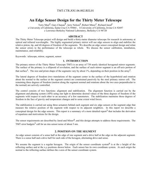
An Edge Sensor Design for the TMT - Thirty Meter Telescope

TMT.CTR.JOU.06.002.REL01
An Edge Sensor Design for the Thirty Meter Telescope
Terry Mast a , Gary Chanan b , Jerry Nelson a , Robert Minor c , Richard Jared c
a University of California, Santa Cruz CA 95064 , b University of California, Irvine CA 92697
c Lawrence Berkeley National Laboratory, Berkeley CA 94720
ABSTRACT
The Thirty Meter Telescope project will design and build a thirty-meter diameter telescope for research in astronomy at
optical and infrared wavelengths. The highly segmented primary mirror will use edge sensors to align and stabilize the
relative piston, tip, and tilt degrees of freedom of the segments. We describe an edge sensor conceptual design and relate
the sensor errors to the performance of the telescope as whole. We discuss the sensor calibration, installation,
maintenance, and reliability.
Keywords: telescope, mirror, segment, sensor
1. INTRODUCTION
The primary mirror of the Thirty Meter Telescope TMT) is an array of 738 nearly identical hexagonal mirror segments.
The surface of the primary is a ellipsoid of revolution, and the surface of each mirror segment is an off-axis portion of
that surface 1 . The size and prism shape of the segments vary by about 1%, depending on their position in the array 2 .
The lateral degrees of freedom (two translations of the segment center in the surface of the hyperboloid and rotation
about the normal to the surface at the segment center) are constrained passively by the steel primary mirror cell. The
remaining three degrees of freedom (motion along the segment normal and rotations about the two axes perpendicular to
the normal) are actively controlled.
The control consists of two functions: alignment and stabilization. The alignment function is carried out by the
alignment and phasing system (APS) using star light to determine desired values of the three degrees of freedom of the
segments with respect to each other to an accuracy of a few nanometers. The stabilization maintains those degrees of
freedom in the face of gravity and temperature changes and to some extent wind forces.
The stabilization is carried out using three actuators behind each segment and six edge sensors at the segment edge that
measure the relative position of the segment with respect to its adjacent neighbors. In this report we describe a
conceptual design for the edge sensors. This report is a summary of a more detailed report 3 that includes the derivation
of equations and motivations for the design.
The sensor requirements are described by Jared and Minor 4 , and this design attempts to address those requirements. The
TMT error budgets 5 call for an rms sensor noise of about 5 nm.
2. POSITION ON THE SEGMENT
An edge sensor consists of a sense half at the edge of one segment and a drive half at the edge on the adjacent segment.
There is a sense half and a drive half for each side of the hexagon, alternating drive and sense.
We assume the segment is a regular hexagon. The origin of the sensor coordinate system 6 is at the z height of the
reflecting surface and at the x,y positions shown below. Each sensor has its own coordinate system. At each origin the
normal to the reflecting surface defines the z-axis of the sensor coordinate system.

TMT.CTR.JOU.06.002.REL01
Exaggerated side view of two adjacent segments.
Bold arrows are normals to the reflecting surface.
The x axis is parallel to the hexagon side,
and directions of positive x are shown below.
y M1
z SEN
drive
sense
origin
y SEN
x M1
The hexagon sides shown above are at the mid-planes of the inter-segment gaps.
y drive sense
M1
y
drive
e
sense
β
x M1
The distance e is identical for all sensors and all segments. The angle β is given by
the center-to-vertex distance of segment j.
tan β = √3e/(2a j
− e) ; where a j
is
3. OVERALL DESCRIPTION
Each sensor uses a change in the charge on a capacitor to measure a linear combination of
1) a change in the relative height (δz) of the two adjacent segments and
2) a change in the dihedral angle (δω) between the two adjacent segments.
z
x
sense
plate
drive plate 1
Capacitor plates (not to scale).
The sense plate is on one segment and the drive
plates are on the other. Each half (drive or sense) is a
single block of low thermal expansion glass-ceramic
plated with capacitor plates. Each block is attached
to the back of a segment.
drive plate 2

TMT.CTR.JOU.06.002.REL01
4. SENSITIVITIES
We describe the sensor sensitivity to all six degrees of freedom of one segment with respect to the adjacent segment;
translations δx , δy , δz and rotations δθ x
, δθ y
, δθ z
. For a simple capacitor C = Q/V = εA/g , where C = capacitance,
Q = charge, V = voltage, ε = 8.85e −12 (farads/m), A = plate area, g = gap between plates.
The proposed sensor geometry is shown below (not to scale).
end view
ω
z
y
x
side view
segment
h segment
t
L sensor
drive plate a 1
g 1
g 2
sense
plate
drive plate 2
b 1
2f
b 2
2B
h block
drive 1
voltage
drive 2
voltage
Center Line
The basic concept is similar to the capacitive sensor used for the Keck telescopes; a vertical motion of one segment will
increase one capacitance while decreasing the other. This will be highly linear in the displacement and dihedral angle
changes for the small changes that will occur. We calculate the detailed geometry of the proposed TMT sensor design
using the two simplifying assumptions.
1. The capacitance is that of a simple capacitor in air. This is not strictly true since the glass-ceramic substrate
has a dielectric constant. This reduces the capacitance by a factor up to about 2; calculated using the simulation code
Maxwell. Consequently, to avoid this reduction we propose here to add ground planes to all sides of the sensor block
with a 1 to 2 mm gap between the ground planes and active capacitor plates. Simulation of this configuration gives
capacitances and sensitivities that agree within 1% of those calculated using the simple formulas used above.
2. The dielectric constant of the glass-ceramic substrate will enhance the coupled capacitance between the two
drive plates. For the separation of the plates assumed below (4 mm) the coupled capacitance is small.
Sensitivity to relative segment motions δz and δθ x
(= δω)
Although the design calls for symmetry in the plate dimensions, fabrication errors will result in small differences leading
to non-zero values for Δ∆B, Δ∆ω, and ∆G defined as follows.
Distances B and ∆B:
b 1
= B − f + (∆B + δz) and b 2
= B − f − (∆B + δz))
Dihedral angle between segments: ω = ∆ω + δω
Distances G and ∆G:
g 1
= G + ∆G + (L sensor
−f−b 1
/2)(∆ω + δω)
g 2
= G + ∆G + (L sensor
+f+b 2
/2)(∆ω + δω)
Drive voltages V and ∆V: V 1
− V 2
= 2V and V 1
+ V 2
= 2∆V
The sensor reading R = Q 1
+ Q 2
= [2εaBV/G] [∆V/V + (∆B+δz)/B + (B+f)(∆ω+δω)/2G)]

TMT.CTR.JOU.06.002.REL01
The alignment/phasing processes tune ∆V (= V offset
) to achieve ∆V/V + ∆B/B + (B+f) ∆ω/2G) = 0
Afterwards the segment stabilization system uses the reading change δR to move the segments to correct small non-zero
values δz and δω.
δR = [2εV/G] [ δz +(B(B+f)/(2G)) δω ]
Define L effective
= B(B+f)/(2G) ⇒ δR = [2εV/G] (δz + L effective
δω)
Sensitivity to δθ z
A rotation about the z axis to first order will not change the average gap and will have no effect on the final charge
developed on the sense plate. The next order effect is negligibly small (δC/C ~ 0.2 x 10 −10 ).
Sensitivity to δθ y
Consider the segment rotated about y, such that the other sensor on the same segment edge reads a maximum of it’s
operating range. A calculation for our proposed sensor shows the false reading generated by this rotation is ~10 −14 m,
negligibly small.
Sensitivity to δx
The drive plates are intentionally wider than the sense plate in order to make the output insensitive to small δx. Second
order fringe-field effects are expected to cancel and only negligibly small third order fringe-field effects will contribute.
A potentially significant δx sensitivity is created if a fabrication/installation error introduces a difference in θ y
between
the sense plate and the drive plates, θ y-d-s
. Then a gravity-induced or temperature-induced change in x (δx) causes a
reading change corresponding to δz false
= δx θ y-d-s
. Assume the sense plate has width = 30 m and is applied to an
accuracy of 10 microns rms at the corners with respect to the block then θ y-d-s
= 0.010/15 = 7 x 10 −4 radians rms. If
δx = 0.1 mm. ⇒ δz false
= 70 nm rms. This is a large effect, and will be removed using a fit to all gap measurements to
establish the value of δx to < 5 microns and a fit to temperature and zenith angle to refine this to δx to < 1 micron,
resulting in δz false
< 0.7 nm rms.
Sensitivity to δy (= gap change = δG)
Since the gap (G) will vary with gravity and temperature (resulting in changing the sensor output), we also need to
measure G. We address below 1) the sensitivity to gap changes, 2) the expected size of the changes, 3) a method to
measure the gap, and 4) the processing of the measurements. The gap measurement will be used to digitally correct the
reading δR.
1) Sensitivity to gap changes. There are three ways a change in the gap (δG) affects the reading δR.
• It changes the sensitivity to δz. δR/δz = 2εaV/G δ(δR/δz) = (δR/δz)(−δG/G)
• It changes the sensitivity to δω δR/δω = 2εaVB(B+f)/(2G 2 ) δ(δR/δω) = (δR/δω)(−2δ/G)
• It means the offset voltage is erroneous
V offset
= −V[∆B/B + (B+f)∆ω/(2G)] δV offset
= −V(B+f)∆ω δG/(2G 2 )
δR = 2εBδV offset
/G = −2εVB(B+f)∆ω δG/(2G 3 )
where ∆ω is the dihedral angle between segments after segment installation.
In terms of a comparable δz δz = −B(B+f)∆ω δG/(2G 2 )
2) Expected size of gap changes.
Temperature-induced: If the cell temperature changes by 10 o C, then δG = 125 microns.
If we assume a rate of 1 o C per hour, then δG/dt = 3.5 nm/second.

TMT.CTR.JOU.06.002.REL01
Gravity-induced: If the primary mirror moves by ~10 mm, and we assume that 10%
is differential, then δG ~ 1mm/30m = ~ 30 microns.
If this happens during a zenith to horizon slew in 2 minutes, then δG/dt = 250 nm/second.
We assume: • a maximum gap change of 150 microns ⇒ δG/G = 0.15/2.0 = 0.075
• a maximum rate of 250 nm/second.
Using these values
• Change in sensitivity to δz. δG/G = 0.075
• Change in sensitivity to δω. 2δG/G = 0.15
These changes in sensitivity (1.075 and 1.15) change the convergence rate of the segment stabilization control.
However, they are minor compared to gain of the control system (typically 0.2 to 0.1).
• Erroneous offset voltage. In terms of a comparable δz, δz = −B(B+f) ∆ω δG/(2G 2 )
⇒ We want δG/G < δz max
2 G/[B(B+f)∆ω max
]
We want stability to δz < 3 nm. The δG/G limit then depends on the installation error ∆ω max
.
For a maximum installation error ∆z max
, the following diagram shows an extremely conservative estimate of
∆ω max
. The diagram assumes the extremely unlikely configuration with all four sensors at the maximum ∆z max
.
∆ω max
= 2 ∆ max
/1.04 m
1.04 m
If ∆ max
=30 microns, then ∆ω max
= 6 x10 −5 radians. If B = 15 mm, f = 2 mm, G = 2 mm, then δG/G < 1/1275.
We require the gap to be measured to this level from one alignment/phasing procedure to the next; ~several weeks.
3) Measuring the gap.
The sensor electronics are described below. We will measure the gap by modifying at 20Hz the drive voltages for 1
pulse of the 10 kHz square wave; equal to 2 of the 1000 charge pulses (both edges of the square wave give a charge
pulse), and then average the 2 pulses.
+V
V 1
+V g
V 2
−V
The modification will reverse the sign of V 2
and reduce the voltage to V g
= 1.0 V to prevent saturation.
The reading during the gap measurement using a single pulse will be R = Q 1
+ Q 2
= εV g
2(B−f)w/G.
Assume B = 0.015 m, f = 0.002 m, w = 0.030 m, G = 0.002 m, ε = 8.85 x 10 -12 , V g = 1 volts. Then
R = 3.5 x 10 -12 Coulombs = 2.2 x10 7 electrons, and averaging 2 charge pulses gives 4.4 x10 7 electrons. The error
from electron statistics alone is δG/G = δR/R = 1/N 1/2 e = 1/9300. For the error from ADC bit size assume a signal
of 2000 counts for the 2 mm gap, and assume the rms error for 1 LSB = 12 −1/2 = 0.29 ⇒ δG/G = 1/6900.
Both of these are smaller than our goal of 1/1275, thus averaging only two charge pulses is sufficient.
4) Processing the Measurements
We will use the local temperature (T), the elevation encoder reading (el), and the sensor gap measurement (G), to
create a local sensor-by-sensor correction to the raw sensor reading.
[We will also use the APS measurements, the gap measurements, the elevation encoder reading (el), and the
temperature measurements (T) to create a Global look-up table of desired sensor readings as a function of T
and el.]
+V g

TMT.CTR.JOU.06.002.REL01
With 4212 gap measurements and (3*738−3) in-plane segment degrees of freedom, we are highly over constrained.
We will make a fit to the ensemble of gap measurements to determine their consistency and the measurement error.
We will use the fit to all gap measurements to establish the best estimate of the gap for each sensor and an estimate
of the temperature of the mirror cell. Smooth functions of el and T will be fit to the measurements made at many
values of el and T, and a correction for each sensor will be constructed from the fits. We expect the residuals to the
lookup tables will be random and thus correspond to random sensor noise. We want the residuals to be less than ~3
nm rms.
Temperature
In addition to direct temperature measurements, we will also use the average gap measurement as a measure of the
average cell temperature. The lowest order effect of temperature is a uniform change in the temperature of the
mirror cell. The gap change is the same for all gaps (uniform expansion or contraction of the cell). Using the
average of all gap measurements we will create a highly precise lookup table versus temperature. The error of each
sensor gap (σ G
) can be made small by averaging over time. In addition, the error on the average over all sensors
further reduces the measure of this single mode: σ G
/4212 1/2 = σ G
/65 . If the sensor readings were not corrected for
this, then the readings would be erroneously interpreted as a focus-mode deformation of the primary mirror array.
5. CAPACITOR PLATE DIMENSIONS
Drive Plate Design
Width (w drive
) To make the reading insensitive to motions along the x-axis (δx),
we use a drive plate width that extends beyond the sense plate by 5 mm (see below).
Height (h drive
) To accommodate the sensor range in z and make the reading insensitive to rotations about the y-axis
(δθ y
), we use drive plate heights that are smaller than the sense plate by 3.0 mm (see below).
Drive Plate Separation (2f) To maintain a small capacitive coupling between the two drive plates,
we use a plate separation of 4 mm corresponding to f = 2 mm.
Sense Plate Design
In the design calculations we have assumed the simple capacitance formulas and assume ground planes surround the
capacitor plates. A simulation program “Maxwell” confirms the simple formulas are accurate.
Width (w sense
)
We compare the δz sensitivity with the sensors being used on the Keck telescopes.
TMT/Keck = [w
tmt
sense
V
tmt /G
tmt ] / [A
keck V
keck /(G
keck )
2 ]
A keck = 30 x 30 = 900 mm 2 V keck = 6.74 volts G keck = 4 mm G tmt = 2 mm
We propose here for the TMT w
tmt
sense
= 30 mm, V
tmt = 6 volts.
TMT/Keck = ~1/4
Height (h sense
)
control-stabilization :
The maximum δz range is ~ 2 (a/t) act max
,where a = 0. 6 m, t = 0.31 m, act max
= 3.4 mm is the maximum
actuator range maximum δz ~ 15 mm. However, Even if the sensors saturate the stabilization will converge.
control-stabilization :
This is dominated by the need to use focus-mode and three-color mode for alignment.
Focus mode is “edge continuous” so it shouldn’t require δz motions. Three-color mode is used to
• capture pistons for installation misalignment errors in sensor alignment lookup table (< 10 microns)
Conclusion: The range must be perhaps a few times the offset range.

TMT.CTR.JOU.06.002.REL01
sensitivity to dihedral angle δω.
Assume G = 2 mm, B = 15 mm (h sense
= 2B), f = 2 mm (plate separation = 4 mm)
L effective
= B(B+f)/(2G) ⇒ L effective
= 63.8 mm
5
50
5
Mirror
10
mm
dimensions in millimeters
17.5
Sense pad 30 x 30
52 4
30
17.5
mm
Drive pads 17.5 x 40
3
50
With these dimensions the capacitance from the overlap with one drive plate is 1.73 pF.
6. MECHANICAL DESIGN
The sensor substrate is a rectangular block of glass-ceramic or ULE with dimensions in the table below.
All sides are polished to relieve stress. All edges are beveled.
Three raised feet on each block contact the shined spherical back of the segment. A rare earth magnet is bonded to the
block. This attracts a similar magnet bonded to the back of the segment and holds the block in position on the segment.
The block may be positioned using nylon pins protruding from two blind holes drilled into the back of the segment. One
pin seats in a blind hole in the block and the other rests against the edge of the block. Alternately, registration blocks
attached to the mirror back may be used, thus eliminating the need for holes in the mirror.
Three holes through the block thickness provide paths for wires to connect to the sense and power plates. Thus all
electronics connect to the back of the sense block.
A method to keep the gap isolated from dust, water, and water vapor is critical to the performance. We leave a space
between the plate side of the block and the segment of 5 x 5 x 50 mm for a barrier we call the “gaiter”. A flexible torus
of material can be inserted through the gap and connected around each block in this space. The figure below illustrates
the concept.

TMT.CTR.JOU.06.002.REL01
A collapsed gaiter might be stored on one block of one
side of the sensor for segment installation, and then for
segment use it might be deployed across the gap either
manually or using air pressure or an electromagnet. An
explicit design is remains to be created.
The mechanical dimensions follow.
Each Block Sense Block (mm)
dimensions (mm) feed through hole (1)
length (along edge of segment) 50 diameter 2
depth (extending behind segment) 45 sense plate
(boot space 5, capacitor space 40) Z height 30
thickness 20 X length 30
(15 mm at boot space)
edge bevels (12) 0.3
feet (3)
length 4
widths (2) 2
width (1) 4
height 1
hole for rare earth magnets
diameter 10 Drive Block (mm)
depth 7 feed through holes (2)
hole for positioning pin diameter 2
diameter 3 drive plates (2)
Z height 17.5
X length 40
block volume (m^3)
4.5E-05
block mass (kg) 0.114
Comments.
Feet (3): The compression induced by the magnet force will not compress the feet to match the curved segment
surface. The feet must be polished on a curved tool (radius ~ 60 m) to seat properly.
In addition, the feet heights must match the spherical surface slope and the normal at the gap for the block to be
at an angle such that the gap is uniform. The spherical surface slope at the edge is ~a/k = 0.6/60, and over the
block thickness (20 mm) gives a difference in feet height of 200 microns. The nominal height is 1 mm, but the
actual heights must provide this 200 micron difference.
Surfaces: all are fine ground
Capacitor plates: coating: 0.5 microns of gold over 0.05 microns of chrome
Magnets: rare earth magnets: minimum required force ~ 15 X sensor mass = 1.5 kg ~ 15 N
We assume two magnet pairs/block with each magnet for a total of (2)(12)(738)(7/6) = 20,700 magnets.

TMT.CTR.JOU.06.002.REL01
segment back surface
boot
space
front view
end view
blind hole
through hole
for wire to
sense plate
sense
plate
blind hole
top view
rare earth
magnets
positioning
rods
7. ELECTRONICS (DESIGN, RANGE, LINEARITY)
Design
The next three drawings show an initial design of the proposed sensor electronics.
The sensor is connected to the Pre-Amplifier by a coax cable (0.3 to 0.6 m long). The electronics at the sensor fit on a 50
x 50 mm board that is permanently attached to the segment.
• Readout at 20 Hz has 1000 ADC data samples:
998 samples are summed to measure position/tilt and 2 samples are used to measure the gap.
Both numbers are read at 20 Hz.
• The gap calibration pulse is used to obtain the ADC value for a gap of 2 mm.
• In “Fast Data Capture” mode the sensor is read at 400Hz, is locally stored and readout at a later time.

TMT.CTR.JOU.06.002.REL01
Electronics Overview
Sensor 1 of 6 shown
Mirror Sensor Electronics 1 of 123
Sensor
Connector
for drives 6 ea.
A B C
Sensor
Charge
Electronics
at
Sensor
contains:
Preamp
Shaper Amp
Driver
Goal 300 mw
Position
and Tilt
Sensor Analog
Gap Calib Pulse
DC Power
Gap
Connector
6 PreAmps
Electronics
at
Mirror
Support for 6
sensors
contains:
6 ADCs
6 DAC sets
1 FPGA
Sensor data
Oscillator
Sync
Read/write
Drive 1
Drive 2
Connector
6 drive
sets
Electronics at Sensor
Pre-Amplifier
RC(CR)2 Shaping Amplifier
~ 4 micro-seconds Cable driver
A
B
Sensor Analog
Sensor
Charge
Calibrated Capacitor
+/- 6 V DC to all
DC Power
Gap Calib Pulse

TMT.CTR.JOU.06.002.REL01
Electronics at Mirror
B
Sensor Analog
6 ea Sensor Support, BLC and ADC
ADC 16bit
DC Power
ADC & BLC Timing
Gap Calib Pulse 6 ea
6 ea Sensor Drive Generation
6 set SW
Gap
Drive 1 6 ea
Gap Calib DAC
1 ea
Gap DAC 1 ea
Offset DAC 6 ea
0.1 VGMax
to –0.1 VGMax
R/W
R/W
R/W
FPGA Contains:
1 Generation of
Switch Control
for position/tilt, gap, &
gap calibration
2 R/W to DACs
3 Generation of 10kHz
4 Timing of ADC
5 Integration of all pulses
in 20 Hz readout period
6 Capture & integration of
fast data stream (400Hz)
7 Readout of sensor
position/tilt and gap data
8 Readout out of gap
calibration pulse
C
Sensor data
Oscillator
Sync
Read/write
Drive 2
Position
and Tilt
6 ea
Gain DAC 1 ea
0 to VGMax
Switch Control
R/W
DC Power
Range
Using standard fixtures we will measure the position of the plates with respect to the reflecting surface after each sensor
is attached to the segment. The initial offset voltages will be determined using these measurements. We assume the rms
measurement error is 10 microns. To accommodate measurement errors and allow the phasing measurement to
“capture” all segments, we assume the electronics requires a full range (in possibly a “coarse” mode) of ±30 microns.
Linearity
We assume the non-linearity to be dominated by the non-linearity in the final ADC. Non-linearity caused by fringe fields
and substrate dielectric constant is negligible. Commercial ADC’s with 16 bits advertise a non-linearity of

TMT.CTR.JOU.06.002.REL01
8. SENSOR NOISE
We assume a square wave pulse rate of 10kHz. We assume the averaging rate for segment stabilization will be 20 Hz
(giving (10kHz*2)/20 Hz = 1000 charge pulses per average) and for diagnostics (called “fast data capture “ mode at
Keck) will be 400 Hz (giving 50 pulses per average).
For segment stabilization, the telescope error budget calls for a sensor electronic noise corresponding to ~3 nm rms δz.
For δz = 3 nm, δC = 0.273pf/mm from Maxwell simulations and V = 6V, the charge from a single 3 nm pulse is
δQ = δCV = 31 electrons.
The noise will be dominated by noise in the pre-amp, and we have determined using both simulation and calculation a
noise of 90 electrons rms for each charge pulse. Since alternate pulses have opposite signs, the base line is removed, and
the signals from 1000 pulses are added. The signal-to-noise ratio is S/N = (3 1electrons * 1000)/(90 electrons * 1000 ½ )
= 11 corresponding to 0.3 nm rms. The Keck sensor electronics noise is < 1 nm rms 7 .
9. SENSOR NOISE PROPAGATION TO PRIMARY MIRROR
A detailed description of the effect of sensor noise on the shape of the full primary mirror is given in Reference 3.
A fundamental result is
80%ΕΕ = σ s
[0.0065] with 80%ΕΕ in arc seconds on the sky and σ s
in nm
The TMT error budget calls for 80%ΕΕ < 0.030 arc seconds, requiring σ s
< 4.6 nm. This gives rms surface S rms
= 58
nm and rms wavefront W rms
= 116 nm. The implication of this value for the sensor requirements depends on the TMT
control bandwidth. If we assume a bandwidth (BW) = 0.3 Hz and a white noise spectrum, then the required sensor noise
(S noise
) is given by 8
S noise
= σ s
/[(π/2) BW] 1/2 yielding S noise
< 6.7 nm/√Hz 1/2
10. POSITION SENSITIVITY
We assume the magnets will hold the sensor in position during operations. The following are the tolerances for
installation of the block on the back of the segment.
Δx < ± 0.5 mm To not add fringe field effects to capacitances
Δy < ± 0.1 mm To not significantly change the gap
Δz < ± 0.03 mm
Δθ x
< ± 3.0e-3 rad (0.2mm/66mm) To not require too large an offset ΔG
Δθ y
< ± 2.5e-3 rad (0.5mm/200 mm) To not add fringe field effects
Δθ z
< ± 5.0e-4 rad (0.1mm/200 mm) To not add fringe field effects
11. GRAVITY SENSITIVITY
Gravity changes from zenith to horizon will change the sensor reading, resulting in relative motions of the sense and
drive blocks, in two ways:
• deformation of the segments
• bending and tilt of the sensor
A priori we expect the first to dominate, since the drive and sensor block will move under lateral gravity in opposite
directions. We expect the bending and tilt of the sensors to be in the same direction canceling the effect on the sensor
reading.
Deformation of the Segments: Axial gravity
The axial component of gravity acting on the sensor blocks will deform the segment. To first order, this will be
corrected by re-optimizing the positions of the whiffletree/segment attachment points. Any residuals will be corrected at

TMT.CTR.JOU.06.002.REL01
the zenith using ion figuring. This will result in a surface deformation as the zenith angle increases. However the
overall error budget increases with zenith angle, and this particular term can increase substantially. We anticipate that
his axial gravity term will readily meet the error budget.
Deformation of the Segments: Lateral gravity
Because the sensors extend in back of the segment, lateral gravity will induce a moment on the edges of the segments.
Relative motions of the sensor blocks will be in the same direction in the plane of the segments, but in opposite
directions normal to the segments.
g
We will make a finite element calculation to estimate the magnitude of this effect. However, it will be removed using
the APS-generated lookup table (a function of zenith angle). In addition, the error budget allows the error to increase
substantially with increasing zenith angle. The residual error from the lookup table will make a negligible contribution
to the error budget.
Bending and tilt of the sensor
Under gravity loads in the x and y directions the body will bend and the feet will compress. Since the drive and sense
halves are identical, the effects will cancel and have a negligible effect on the reading. In addition, if there is any
residual effect, it will be smoothed with a fit to a function of elevation angle and be removed in the APS-generated
lookup table.
We have calculated the magnitude of the bending and tilting effects that will be cancelled. The sensor bending under its
own weight is for gravity in the x and y direction is 0.3 and 2.2 nm respectively.
At elevation angle = 0 the sensor will tilt since the force on one foot will increase (δF) and on the other decrease (−δF).
Balancing the moment gives a maximum displacement of 10.2 nm. The force applied to each foot by the magnet is
about 15 times the sensor weight; F axial
= 0.114 (9.8) 15 / 2 = 8.4 N
At the horizon, the force on the upper foot is reduced by 1.8 N (~20%) and the force on the lower foot is increased by 1.8
N. The friction between the feet and the segment must be adequate to prevent creep motion of the sensor as the
telescope is repeatedly moved over a large range in zenith angle.
12. TEMERATURE SENSITIVITY
The mechanical sensor is made of low thermal expansion glass ceramic with a CTE that will closely match the CTE of
the segment. Small differences in CTE might lead to a sensitivity up to ~10 nm/ o C, and this will be removed by
calibration. The residual will not contribute significantly to the temperature sensitivity. The temperature sensitivity of
the readout electronics depends on the selection of components. As a guide, the rms temperature sensitivity of the Keck
sensors 7 is about 0.3nm/ o C.
13. HUMIDITY SENSITIVITY
We do not yet have a definitive understanding of capacitive sensor sensitivity to humidity.
• Observers at Keck have never suggested that the humidity degrades the performance.
• Recent laboratory tests of a Keck sensor show a sensitivity to humidity that depends on the nature of the
process used to clean the gold surfaces. Gold has a high free surface energy, and it condenses water with a low free
energy surface. Gabor Somoraji (UC Berkeley) has suggested the possibility of coating the gold with a hydrocarbon or
Teflon, and we will investigate this possibility.

TMT.CTR.JOU.06.002.REL01
14. POWER
Our goal is to have the power radiated by each sensor and its electronics to be < 300 mW. In addition, we require that
the electronics/software allow a complete recovery from a power loss of the settings at the time of the loss. A full
electronics design is being created to meet these requirements.
15. DRIFT WITH TIME
The sensors are required to not drift during the periods between segment alignment/phasing procedures, roughly every
six weeks.
In addition, since we will want to use the array as soon after segment exchange as possible, we have set a goal for the full
sensor system to settle to its final value in less than four hours. We expect that during segment exchange the mechanical
part of the sensor will have been undisturbed from many hours and will have a very small settling time. The electronics
should be largely insensitive to temperature, and we also expect a small settling time.
16. MAINTENANCE
There are three categories of activity that will affect the sensor reading and require a calibration using the APS.
1. Sensor removal and replacement
2. Segment surface cleaning
3. Segment removal, coating, and replacement
1. Sensor removal and replacement
The exchange of a sense block, drive block, or the electronics for a sensor will require one or more measurements by
the APS to re-establish the desired sensor reading.
2. Segment surface cleaning
The cleaning of a segment surface with CO 2
or other agents can potentially affect a sensor reading. This will
require APS measurements to confirm the segment cleaning process does not affect the desired sensor reading. If
the cleaning process has been repeatedly shown to not affect the reading, the use of the APS after cleaning can be
discontinued.
3. Segment removal, coating, and replacement
The effect of the sensor on the coating chamber and the effect of the coating process on the sensor need to be
thoroughly proven and understood. Potential concerns include the heat generated by the segment coating process,
out-gassing of either the sensor or the segment and it’s support, and changes in the sensor’s gold coating.
Removal and replacement of a segment will change the gap (∆G). This alone will require measurements by the APS
to re-define the desired sensor reading.
Removal and replacement of a segment will change the values of ∆z and ∆ω. A database of matching drive block
and sense block serial numbers may be used to improve the efficiency of APS measurements.
17. RELIABILITY
The piston, tip, and tilt degrees of freedom of the 738 segments are actively controlled by 2214 actuators and 4212
sensors. Thus there is extensive redundancy in the sensor measurements. At any one time many sensors could be
deleted from the system, and the stabilization performance would not significantly degrade. The Keck telescopes
typically operate with several sensors deleted from the control algorithm.
ACKNOWLEDGEMENTS
The authors gratefully acknowledge the support of the TMT partner institutions. They are the Association of Canadian
Universities for Research in Astronomy (ACURA), the Association of Universities for Research in Astronomy (AURA),
the California Institute of Technology and the University of California. This work was supported, as well, by the Canada
Foundation for Innovation, the Gordon and Betty Moore Foundation, the National Optical Astronomy Observatory,
which is operated by AURA under cooperative agreement with the National Science Foundation, the Ontario Ministry of
Research and Innovation, and the National Research Council of Canada.

TMT.CTR.JOU.06.002.REL01
REFERENCES
The central archive of TMT documents (Docushare) is at tmt.org. TMT Reports and Technical notes are available at
tmt.ucolick.org
1. Mast, T., J. Nelson, and G. Sommargren, “Primary Mirror Segment Fabrication for CELT”, TMT Report No. 5,
Proceedings of the SPIE, 4003 (June 2000), document archive Docushare CEL.OPT.JOU.00.001.REL01
2. Mast, T. and J. Nelson. “TMT Primary Mirror Segment Shape” TMT Report No. 58 (November 2004) document
archive Docushare TMT.OPT.TEC.04.001.REL01
3. Mast, T., Gary Chanan, Jerry Nelson, Robert Minor, Richard Jared “An Edge Sensor Design for the TMT” TMT
Report No. 70 March 2006
4. Jared, Richard and Robert Minor, “TMT Position and Tilt Sensor Requirements” document archive Docushare
TMT.SEN.SPE.05.001.REL02 (October 2005)
5. Mast, T. and J. Nelson , “Image Size and Wavefront Error Budgets” TMT Report No. 10, document archive
Docushare TMT.OPT.TEC.05.024(,025, and 026).DRF01)
6. Mast, Terry , George Angeli, and Scott Roberts “TMT Coordinate Systems”, TMT Report No 67, document archive
Docushare TMT.SEN.TEC.05.016.DRF04 (2005)
7. Jackson, H.G. and T. T. Shimizu, (Position Sensor Electronics for the Ten Meter Telescope), Keck Observatory
Technical Note No. 224 (April 1987) (LBL-23383)
8. MacMartin and Chanan, Control of the California Extremely Large Telescope Primary Mirror,
TMT Report No. 40, 2002, TMT document archive Docushare CEL.CTR.TEC.02.001.REL01