Magnetic susceptibility of the two-dimensional Ising model ... - LMPT

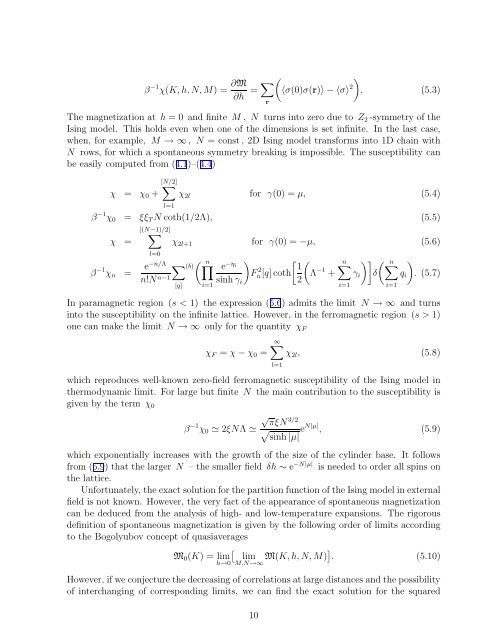
β −1 χ(K, h, N, M) = ∂M
∂h = ∑ r
(〈σ(0)σ(r)〉 − 〈σ〉 2 )
. (5.3)
The magnetization at h = 0 and finite M , N turns into zero due to Z 2 -symmetry of the
Ising model. This holds even when one of the dimensions is set infinite. In the last case,
when, for example, M → ∞ , N = const , 2D Ising model transforms into 1D chain with
N rows, for which a spontaneous symmetry breaking is impossible. The susceptibility can
be easily computed from (4.1)–(4.4)
χ = χ 0 +
[N/2]
∑
l=1
χ 2l for γ(0) = µ, (5.4)
β −1 χ 0 = ξξ T N coth(1/2Λ), (5.5)
χ =
[(N−1)/2]
∑
l=0
β −1 χ n = e−n/Λ
n!N n−1 ∑
χ 2l+1 for γ(0) = −µ, (5.6)
[q]
(b) ( n∏
i=1
) [
e −η i 1
F 2
sinh γ
n[q] coth Λ
i 2(
−1 +
n∑
i=1
( n∑
γ i
)]δ q i
). (5.7)
i=1
In paramagnetic region (s < 1) the expression (5.6) admits the limit N → ∞ and turns
into the susceptibility on the infinite lattice. However, in the ferromagnetic region (s > 1)
one can make the limit N → ∞ only for the quantity χ F
∞∑
χ F = χ − χ 0 = χ 2l , (5.8)
which reproduces well-known zero-field ferromagnetic susceptibility of the Ising model in
thermodynamic limit. For large but finite N the main contribution to the susceptibility is
given by the term χ 0
√ πξN
β −1 3/2
χ 0 ≃ 2ξNΛ ≃ √ e N|µ| , (5.9)
sinh |µ|
which exponentially increases with the growth of the size of the cylinder base. It follows
from (5.9) that the larger N – the smaller field δh ∼ e −N|µ| is needed to order all spins on
the lattice.
Unfortunately, the exact solution for the partition function of the Ising model in external
field is not known. However, the very fact of the appearance of spontaneous magnetization
can be deduced from the analysis of high- and low-temperature expansions. The rigorous
definition of spontaneous magnetization is given by the following order of limits according
to the Bogolyubov concept of quasiaverages
l=1
M 0 (K) = lim
h→0
[
lim
M,N→∞ M(K, h, N, M)] . (5.10)
However, if we conjecture the decreasing of correlations at large distances and the possibility
of interchanging of corresponding limits, we can find the exact solution for the squared
10