Magnetic susceptibility of the two-dimensional Ising model ... - LMPT
Magnetic susceptibility of the two-dimensional Ising model ... - LMPT
Magnetic susceptibility of the two-dimensional Ising model ... - LMPT

You also want an ePaper? Increase the reach of your titles
YUMPU automatically turns print PDFs into web optimized ePapers that Google loves.
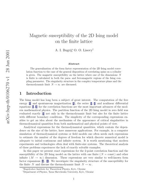
<strong>Magnetic</strong> <strong>susceptibility</strong> <strong>of</strong> <strong>the</strong> 2D <strong>Ising</strong> <strong>model</strong><br />
on <strong>the</strong> finite lattice<br />
arXiv:hep-th/0106270 v1 28 Jun 2001<br />
A. I. Bugrij ∗ , O. O. Lisovy †<br />
Abstract<br />
The generalization <strong>of</strong> <strong>the</strong> form factor representation <strong>of</strong> <strong>the</strong> 2D <strong>Ising</strong> <strong>model</strong> correlation<br />
function to <strong>the</strong> case <strong>of</strong> <strong>the</strong> general disposition <strong>of</strong> correlating spins on a cylinder<br />
is given. The magnetic <strong>susceptibility</strong> on <strong>the</strong> lattice where one <strong>of</strong> <strong>the</strong> dimensions N<br />
is finite is calculated in both <strong>the</strong> para- and ferromagnetic regions <strong>of</strong> <strong>the</strong> <strong>Ising</strong> coupling<br />
parameter. The singularity structure in <strong>the</strong> complex temperature plane and <strong>the</strong><br />
<strong>the</strong>rmodynamic limit N → ∞ are discussed.<br />
1 Introduction<br />
The <strong>Ising</strong> <strong>model</strong> has long been a subject <strong>of</strong> great interest. The computation <strong>of</strong> <strong>the</strong> free<br />
energy [1] and spontaneous magnetization [2], <strong>the</strong> series [3, 4] and nonlinear differential<br />
equations [5, 6] for <strong>the</strong> correlation functions are <strong>the</strong> most important advances <strong>of</strong> <strong>the</strong> modern<br />
ma<strong>the</strong>matical physics. The partition function <strong>of</strong> <strong>the</strong> 2D <strong>Ising</strong> <strong>model</strong> in zero field was<br />
evaluated exactly [7] not only in <strong>the</strong> <strong>the</strong>rmodynamic limit but also for <strong>the</strong> finite lattice<br />
with different boundary conditions. The simplicity <strong>of</strong> <strong>the</strong> corresponding expressions enables<br />
to get an idea about <strong>the</strong> mechanism <strong>of</strong> <strong>the</strong> appearance <strong>of</strong> critical singularities in<br />
<strong>the</strong>rmodynamical quantities from both ma<strong>the</strong>matical and physical points <strong>of</strong> view.<br />
Analytical expressions for <strong>the</strong> <strong>the</strong>rmodynamical quantities, which contain <strong>the</strong> dependence<br />
on <strong>the</strong> size <strong>of</strong> <strong>the</strong> lattice, have numerous applications. For example, in a computer<br />
simulation <strong>of</strong> <strong>the</strong>rmodynamical systems or field <strong>model</strong>s one <strong>of</strong>ten needs such expressions<br />
to estimate <strong>the</strong> number <strong>of</strong> <strong>the</strong> degrees <strong>of</strong> freedom for which discrete numerical <strong>model</strong> is<br />
adequate to initial continuous and infinite system. It is worth mentioning that modern<br />
experiments and technologies <strong>of</strong>ten deal with finite-size systems. The <strong>the</strong>oretical analysis<br />
<strong>of</strong> <strong>the</strong>se problems experiences <strong>the</strong> lack <strong>of</strong> exactly solvable examples.<br />
In this paper we present exact expressions for <strong>the</strong> 2-point correlation function and <strong>the</strong><br />
<strong>susceptibility</strong> <strong>of</strong> <strong>the</strong> 2D <strong>Ising</strong> <strong>model</strong> on <strong>the</strong> lattice with one finite (N = const ) and o<strong>the</strong>r<br />
infinite (M → ∞ ) dimension. These expressions are very similar to well-known form<br />
factor expansions [8], [9]. We investigate <strong>the</strong> singularity structure <strong>of</strong> <strong>the</strong> <strong>susceptibility</strong> for<br />
<strong>the</strong> finite N and discuss <strong>the</strong> <strong>the</strong>rmodynamic limit N → ∞ .<br />
∗ Bogolyubov Institute for Theoretical Physics, Kyiv, Ukraine<br />
† Department <strong>of</strong> Physics, Taras Shevchenko University, Kyiv, Ukraine<br />
1
2 Correlation function 〈σ(0, 0)σ(x, 0)〉<br />
The <strong>Ising</strong> <strong>model</strong> on <strong>the</strong> M × N square lattice (Fig. 1) is defined by <strong>the</strong> hamiltonian H[σ]<br />
Figure 1: The numeration <strong>of</strong> <strong>the</strong> sites <strong>of</strong> <strong>the</strong> lattice and <strong>the</strong> variants <strong>of</strong> <strong>the</strong> disposition <strong>of</strong><br />
correlating spins: a) along <strong>the</strong> cylinder axis, b) arbitrary disposition <strong>of</strong> correlating spins on<br />
<strong>the</strong> lattice.<br />
H[σ] = −J ∑ r<br />
σ(r)(∇ x + ∇ y )σ(r),<br />
where <strong>two</strong>-<strong>dimensional</strong> vector r = (x, y) labels sites <strong>of</strong> <strong>the</strong> lattice: x = 1, 2, . . . , M ,<br />
y = 1, 2, . . . , N ; <strong>the</strong> <strong>Ising</strong> spin σ(r) in each site takes on <strong>the</strong> values ±1 ; J > 0 is <strong>the</strong><br />
coupling constant. Shift operators ∇ x , ∇ y act as follows<br />
∇ x σ(x, y) = σ(x + 1, y), ∇ y σ(x, y) = σ(x, y + 1).<br />
The partition function and 2-point correlation function at <strong>the</strong> temperature β −1 are defined<br />
by<br />
Z = ∑ [σ]<br />
e −βH[σ] , (2.1)<br />
〈σ(r 1 )σ(r 2 )〉 = Z −1 ∑ [σ]<br />
e −βH[σ] σ(r 1 )σ(r 2 ). (2.2)<br />
2
The summation in <strong>the</strong>se formulae has to be taken over all spin configurations. We will use<br />
<strong>the</strong> following dimensionless parameters<br />
K = βJ, t = tanhK, s = sinh 2K. (2.3)<br />
We will consider <strong>the</strong> lattice with periodic boundary conditions for both X and Y<br />
directions. This gives <strong>two</strong> equations for ∇ x , ∇ y<br />
(∇ x ) M = 1, (∇ y ) N = 1.<br />
For such boundary conditions <strong>the</strong> partition function (2.1) can be expressed in terms <strong>of</strong> four<br />
summands [7]<br />
Z = (2 cosh 2 K) MN · 1<br />
)<br />
(Q (f,f) + Q (f,b) + Q (b,f) − Q (b,b) , (2.4)<br />
2<br />
where each <strong>of</strong> <strong>the</strong>m is <strong>the</strong> pfaffian <strong>of</strong> <strong>the</strong> operator ̂D (<strong>the</strong> lattice analogue <strong>of</strong> <strong>the</strong> Dirac<br />
operator)<br />
where<br />
̂D =<br />
⎛<br />
⎜<br />
⎝<br />
Q = Pf ̂D, (2.5)<br />
0 1 + t∇ x 1 1<br />
−1 − t∇ −x 0 −1 1<br />
−1 1 0 1 + t∇ y<br />
−1 −1 −1 − t∇ −y 0<br />
⎞<br />
⎟<br />
⎠ . (2.6)<br />
The upper indices (f, b) <strong>of</strong> <strong>the</strong> quantities Q in (2.4) correspond to different types (antiperiodic<br />
or periodic) <strong>of</strong> boundary conditions for <strong>the</strong> operators ∇ x , ∇ y in (2.6):<br />
(∇ (b)<br />
x )M = (∇ (b)<br />
y )N = 1,<br />
(∇ (f)<br />
x )M = (∇ (f)<br />
y )N = −1. (2.7)<br />
When, for example, M ≫ N (i.e. torus is reduced into cylinder), <strong>the</strong>n in <strong>the</strong> right hand<br />
side <strong>of</strong> (2.4) only “antiperiodic” term survives:<br />
Z = (2 cosh 2 K) MN Q (f,f) . (2.8)<br />
Since <strong>the</strong> operator ̂D is translationally invariant, <strong>the</strong> pfaffian (2.5) can be easily evaluated.<br />
After performing <strong>the</strong> Fourier transformation, one has <strong>the</strong> following factorized representation<br />
for <strong>the</strong> partition function (2.8)<br />
Z = 2 MN∏ q<br />
(f,f)<br />
(s 2 + 1 − s · cos q x − s · cos q y ) 1/2 . (2.9)<br />
The upper index (f) in products (or sums hereinafter) implies that <strong>the</strong> components <strong>of</strong><br />
quasimomentum q x and q y in Brillouin zone run over halfinteger values in <strong>the</strong> units 2π/M<br />
and 2π/N respectively; integer values correspond to <strong>the</strong> index (b) . For example,<br />
∏<br />
q y<br />
(f)<br />
F(qy ) =<br />
N∏<br />
l=1<br />
( ) 2π<br />
F<br />
N (l + 1) ,<br />
2<br />
3<br />
∏<br />
q y<br />
(b)<br />
F(qy ) =<br />
N∏<br />
l=1<br />
( ) 2π<br />
F<br />
N l .
The product over one <strong>of</strong> <strong>the</strong> quasimomentum components in <strong>the</strong> right hand side <strong>of</strong> (2.9)<br />
can be evaluated to <strong>the</strong> explicit form, so for <strong>the</strong> partition function one has<br />
Z = (2s) MN/2∏ q<br />
(f)<br />
e<br />
−Mγ(q)/2 ( 1 + e −Mγ(q)) , (2.10)<br />
where <strong>the</strong> function γ(q) is <strong>the</strong> positive root <strong>of</strong> <strong>the</strong> following equation<br />
sinh 2 γ(q)<br />
2<br />
where <strong>the</strong> parameter µ is <strong>the</strong> function <strong>of</strong> s<br />
= sinh 2 µ 2 + sin2 q 2 , (2.11)<br />
sinh µ 2 = 1 √<br />
2<br />
(√ s − 1/<br />
√ s<br />
)<br />
. (2.12)<br />
For q ≠ 0 γ(q) remains positive in <strong>the</strong> whole range <strong>of</strong> variable 0 < s < ∞ , but γ(0)<br />
changes its sign after crossing <strong>the</strong> critical point s = 1. Since <strong>the</strong> product in (2.10) is taken<br />
over fermionic spectrum, which does not contain <strong>the</strong> value q = 0, this does not cause any<br />
problem here. However, <strong>the</strong> ambiguity in <strong>the</strong> definition <strong>of</strong> γ(0) = ±µ leads to <strong>two</strong> different<br />
representations for <strong>the</strong> correlation function.<br />
The sum over spin configurations in <strong>the</strong> right hand side <strong>of</strong> (2.2) for <strong>the</strong> correlation function<br />
can also be written in terms <strong>of</strong> pfaffians [10]. Corresponding matrices, however, are not<br />
translationally invariant. This fact crucially complicates <strong>the</strong> calculations. Never<strong>the</strong>less, <strong>the</strong><br />
evaluation <strong>of</strong> <strong>the</strong> correlation function can be reduced to <strong>the</strong> evaluation <strong>of</strong> <strong>the</strong> determinant<br />
<strong>of</strong> a matrix<br />
〈σ(0)σ(r)〉 = det A (dim) , (2.13)<br />
with considerably smaller dimension dim = dim(r) , defined by <strong>the</strong> distance between correlating<br />
spins. Fur<strong>the</strong>r work is needed to transform <strong>the</strong> representation (2.13) into <strong>the</strong><br />
representation with analytical dependence on distance.<br />
Form factor representation for <strong>the</strong> correlation function <strong>of</strong> <strong>the</strong> <strong>Ising</strong> <strong>model</strong> is <strong>the</strong> most<br />
acceptable from physical point <strong>of</strong> view. First it was obtained in [8] for <strong>the</strong> infinite lattice in<br />
<strong>the</strong> ferromagnetic region (K > K c , s > 1). Later it was extended [9] for <strong>the</strong> paramagnetic<br />
case (K < K c , s < 1). We note that somewhat earlier similar representation for <strong>the</strong><br />
2-point Green function was deduced in [11] via S -matrix approach [12] for a quantum field<br />
<strong>model</strong> with factorized S -matrix (S 2 = −1 ), which is usually associated with <strong>the</strong> scaling<br />
limit <strong>of</strong> <strong>the</strong> <strong>Ising</strong> <strong>model</strong>. The discovery <strong>of</strong> <strong>the</strong> form factor representation for <strong>the</strong> correlation<br />
function has led to <strong>the</strong> whole trend [13] in <strong>the</strong> integrable quantum field <strong>the</strong>ory.<br />
For <strong>the</strong> finite lattice <strong>the</strong> problem seems to be more difficult, but <strong>the</strong> result [14] is even<br />
simpler in a sense. If correlating spins are located along one <strong>of</strong> <strong>the</strong> axes <strong>of</strong> <strong>the</strong> lattice, <strong>the</strong><br />
matrix in <strong>the</strong> right hand side <strong>of</strong> (2.13) is <strong>of</strong> Toeplitz form. For example, when correlating<br />
spins are located along <strong>the</strong> horizontal axis (Fig. 1a), <strong>the</strong>n<br />
〈σ(r 1 )σ(r 2 )〉 = det A (|x|) , r 2 − r 1 = (x, 0), (2.14)<br />
4
|x| × |x| matrix A (|x|)<br />
k,k ′ has <strong>the</strong> elements [14]<br />
A (|x|)<br />
k,k ′ = 1<br />
MN<br />
∑<br />
p<br />
(f,f) e ipx(k−k′) [2t(1 + t 2 ) − (1 − t 2 )(e ipx + t 2 e −ipx )]<br />
(1 + t 2 ) 2 − 2t(1 − t 2 )(cosp x + cosp y )<br />
k, k ′ = 0, 1, . . . , |x| − 1.<br />
, (2.15)<br />
As it was shown in [14] via Wiener-Hopf integral equations technique [7] adjusted to<br />
<strong>the</strong> finite-sized lattice, <strong>the</strong> determinant (2.14) can be evaluated analytically and for <strong>the</strong><br />
correlation function one has<br />
〈σ(r 1 )σ(r 2 )〉<br />
〈σ(r 1 )σ(r 2 )〉<br />
[N/2]<br />
∑<br />
= (ξ · ξ T )e −|x|/Λ<br />
l=0<br />
[(N−1)/2]<br />
∑<br />
= (ξ · ξ T )e −|x|/Λ<br />
g n (x) = e−n/Λ ∑<br />
( (b) ∏ n<br />
n!N n<br />
F n [q] =<br />
n∏<br />
i N . Note an important detail – summation over <strong>the</strong> phase volume<br />
in (2.18) is taken over bosonic spectrum <strong>of</strong> quasimomenta, in contrast with initial fermionic<br />
spectrum, which defines <strong>the</strong> matrix (2.15). The o<strong>the</strong>r quantities in (2.16)–(2.19) are given<br />
by<br />
ξ = |1 − s −4 | 1/4 , (2.20)<br />
∫π<br />
∣ ln ξ T = N2 dp dq γ ′ (p)γ ′ (q) ∣∣∣<br />
2π 2 sinh(Nγ(p)) sinh(Nγ(q)) ln sin((p + q)/2)<br />
sin((p − q)/2) ∣ , (2.21)<br />
Λ −1 = 1 π<br />
0<br />
∫ π<br />
dp ln coth(Nγ(p)/2), (2.22)<br />
η(q) =<br />
1 π<br />
0<br />
∫ π<br />
0<br />
dp (cosp − e −γ(q) )<br />
cosh γ(q) − cosp<br />
ln coth(Nγ(p)/2). (2.23)<br />
“Cylindrical parameters” ξ T , Λ −1 , η(q) explicitly depend on <strong>the</strong> number <strong>of</strong> sites N<br />
5
on <strong>the</strong> base <strong>of</strong> <strong>the</strong> cylinder. Their asymptotic behaviour for N|µ| ≫ 1 is following<br />
ln ξ T ≃ 1 π e−2N|µ| , (2.24)<br />
√<br />
2 sinh |µ|<br />
Λ −1 ≃ e −N|µ| πN<br />
η(q) ≃<br />
4e −N|µ|<br />
(e γ(q) − 1)<br />
(2.25)<br />
√<br />
sinh |µ|<br />
2πN . (2.26)<br />
Outside <strong>the</strong> critical point cylindrical parameters Λ −1 , ln ξ T and η(q) for large N exponentially<br />
decrease and turn into zero for <strong>the</strong> infinite lattice. Finite sums (2.16), (2.17)<br />
transform into series, summation over phase volume in (2.18) is substituted by integration<br />
and in <strong>the</strong> issue <strong>the</strong> form factor representations on <strong>the</strong> cylinder turn into form factor representations<br />
on <strong>the</strong> infinite lattice [8], [9]. For any finite N both expansions – over even n<br />
(2.16) and over odd n (2.17) – are valid in both ferromagnetic (s > 1) and paramagnetic<br />
(s < 1) regions. We remind that we started from <strong>the</strong> determinant (2.14) <strong>of</strong> a |x| × |x|<br />
matrix. The number <strong>of</strong> terms in its formal definition rapidly increases when x grows.<br />
However, <strong>the</strong> form factor representations (2.16)–(2.19) are <strong>the</strong> finite sums for any fixed<br />
N , and <strong>the</strong> number <strong>of</strong> terms does not depend on |x| . This gives a unique opportunity to<br />
verify (2.16)–(2.19) by means <strong>of</strong> comparing with <strong>the</strong> results <strong>of</strong> transfer matrix calculations<br />
for N− rows <strong>Ising</strong> chains. For fixed N <strong>the</strong> dimension <strong>of</strong> corresponding transfer matrix<br />
is equal to 2 N × 2 N . One can find analytically all eigenvectors and eigenvalues if N is<br />
not too large. We have successfully performed such check analytically for N = 2, 3, 4 and<br />
numerically – for N = 5, 6.<br />
3 Correlation function 〈σ(0, 0)σ(x, y)〉<br />
The rigorous derivation <strong>of</strong> <strong>the</strong> form factor representation on <strong>the</strong> cylinder was performed<br />
in [14] only for <strong>the</strong> spins displaced along <strong>the</strong> cylinder axis. We have not yet succeeded<br />
in generalization <strong>of</strong> <strong>the</strong> method for arbitrary disposition <strong>of</strong> correlating spins (Fig. 1b).<br />
Meanwhile, <strong>the</strong> evaluation <strong>of</strong> <strong>the</strong> momentum representation <strong>of</strong> correlation function<br />
˜G(p) = ∑ r<br />
e ipr 〈σ(0)σ(r)〉, (3.1)<br />
or <strong>the</strong> <strong>susceptibility</strong> (which is connected with ˜G(p = 0)) requires explicit dependence on<br />
both components <strong>of</strong> <strong>the</strong> vector r . Form factor representations (2.16)–(2.19) have a transparent<br />
physical content. This allows to make reasonable assumptions for corresponding<br />
generalizations. The above mentioned possibility <strong>of</strong> independent check allows to eliminate<br />
wrong hypo<strong>the</strong>ses and to make correct choice. In principle, when y -component <strong>of</strong> <strong>the</strong> vector<br />
r is not zero, all quantities in (2.16)–(2.19) could change <strong>the</strong>ir form. Corresponding expressions<br />
for free bosons and fermions on <strong>the</strong> lattice prompt one <strong>of</strong> <strong>the</strong> simplest generalizations<br />
– just <strong>the</strong> substitution<br />
e −|x|γ(q) → e −|x|γ(q)−iyq .<br />
6
Really amazing that it is enough. If instead <strong>of</strong> g n (x) (2.18) one uses <strong>the</strong> expression<br />
g n (r) = e−n/Λ ∑(b)<br />
n∏<br />
( e<br />
−|x|γ j −iyq j −η j<br />
)<br />
F<br />
n!N n sinh γ<br />
n[q], 2 g 0 = 1, (3.2)<br />
j<br />
[q]<br />
j=1<br />
<strong>the</strong>n correlation functions (2.16) and (2.17) exactly coincide with transfer matrix results<br />
for N = 2, 3, 4 in <strong>the</strong> whole range <strong>of</strong> variables x , y , K . Numerical calculations confirm<br />
this for N = 5, 6 also. The validity <strong>of</strong> (3.2) is out <strong>of</strong> doubts and we hope that <strong>the</strong> known<br />
answer will simplify <strong>the</strong> problem <strong>of</strong> its rigorous derivation.<br />
Let us illustrate <strong>the</strong> matter by <strong>the</strong> example <strong>of</strong> N = 3 . The expansion (2.16)–(2.17) are<br />
very similar to <strong>the</strong> representation <strong>of</strong> <strong>the</strong> correlation function in terms <strong>of</strong> eigenvalues <strong>of</strong> <strong>the</strong><br />
transfer matrix<br />
〈σ(0)σ(r)〉 = a 1 (y)(λ 1 /λ 0 ) |x| + a 2 (y)(λ 2 /λ 0 ) |x| + · · · , (3.3)<br />
where λ 0 is <strong>the</strong> largest eigenvalue, coefficients a j (y) are given by some bilinear combinations<br />
<strong>of</strong> eigenvectors. To reduce, for example, (2.17) to (3.3), we use <strong>the</strong> following<br />
expressions for cylindrical parameters ξ T , Λ −1 , η(q)<br />
Λ −1 = 1 ( ∑ (f) ∑<br />
)<br />
(b)<br />
γ(q) − γ(q) , (3.4)<br />
2<br />
q<br />
q<br />
∏ ( )<br />
(b) sinh γ(q)+γ(qi )<br />
2<br />
e −Λ−1 −η(q i ) q<br />
= ∏ ( ), (3.5)<br />
(f) sinh γ(q)+γ(qi )<br />
2<br />
q<br />
∏ ( )<br />
(f) sinh 2 γ(q)+γ(p)<br />
2<br />
ξ 4 T =<br />
∏<br />
q<br />
(b) ∏ p<br />
q<br />
(b) ∏ p<br />
(b) sinh<br />
(<br />
γ(q)+γ(p)<br />
2<br />
) ∏<br />
q<br />
(f) ∏ p<br />
(f) sinh<br />
(<br />
γ(q)+γ(p)<br />
2<br />
). (3.6)<br />
One can derive <strong>the</strong>se expressions from (2.21)–(2.23) by <strong>the</strong> substitution <strong>of</strong> <strong>the</strong> integration<br />
variable z = e iq and computing <strong>the</strong> residues after proper squeezing <strong>the</strong> integration contours.<br />
For N = 3 we have from (3.4)–(3.6) and (2.20)<br />
Λ −1 = 1 2[<br />
γ(π) + 2γ(π/3) − γ(0) − 2γ(2π/3)<br />
]<br />
, (3.7)<br />
Finally,<br />
e −Λ−1 −η(q)<br />
ξξ T =<br />
=<br />
sinh γ(0)+γ(π/3) sinh γ(π)+γ(2π/3) sinh 2 γ(2π/3)+γ(π/3)<br />
2 2 2<br />
sinh γ(0)+γ(2π/3) sinh γ(π)+γ(π/3) sinh γ(π/3) sinhγ(2π/3) , 2 2 (3.8)<br />
γ(0)+γ(q)<br />
sinh sinh 2 γ(2π/3)+γ(q)<br />
2 2<br />
.<br />
sinh γ(π)+γ(q) sinh 2 γ(π/3)+γ(q)<br />
2 2<br />
(3.9)<br />
ln(λ 0 /λ 1 ) = Λ −1 + γ(0), (3.10)<br />
ln(λ 0 /λ 2 ) = Λ −1 + γ(2π/3), (3.11)<br />
ln(λ 0 /λ 3 ) = Λ −1 + γ(0) + 2γ(2π/3), (3.12)<br />
7
a 1 (y) = 1 3<br />
a 2 (y) = 2 3<br />
a 3 (y) = 1<br />
64<br />
×<br />
sinh γ(0)+γ(2π/3) sinh γ(π)+γ(2π/3) sinh 2 γ(2π/3)+γ(π/3)<br />
2 2 2<br />
sinh γ(0)+γ(π/3) sinh γ(π)+γ(π/3) sinh γ(π/3) sinh γ(2π/3) , (3.13)<br />
2 2<br />
sinh γ(0)+γ(π/3) sinh γ(0)+γ(π)<br />
2 2<br />
cos(2πy/3), (3.14)<br />
sinh γ(π/3) sinh γ(π/3)+γ(π)<br />
2<br />
1<br />
sinh γ(0)+γ(π/3) sinh γ(π)+γ(π/3) sinh γ(0)+γ(2π/3) sinh γ(π)+γ(2π/3)<br />
2 2 2 2<br />
1<br />
sinh γ(π/3) sinh γ(2π/3) sinh 2 γ(π/3)+γ(2π/3)<br />
2<br />
.<br />
× (3.15)<br />
The transfer matrix 2 3 × 2 3 has 8 eigenvalues, some <strong>of</strong> <strong>the</strong>m are equal. Besides that,<br />
some eigenvectors have zero components. As result, <strong>the</strong> expression for <strong>the</strong> correlation<br />
function (3.3) contains only three (not seven) independent terms. If we take into account<br />
<strong>the</strong> definition (2.11), (2.12) <strong>of</strong> <strong>the</strong> function γ(q) for particular values <strong>of</strong> quasimomentum<br />
q = 0, π/3, 2π/3, π , we get exact correspondence between this three terms and (3.10)–<br />
(3.15).<br />
4 Momentum representation <strong>of</strong> <strong>the</strong> correlation<br />
function<br />
Since we have <strong>the</strong> expression (3.2) for g n (r), which depends on both components <strong>of</strong> r , we<br />
can make <strong>the</strong> Fourier transform. Let us write <strong>the</strong> momentum representation <strong>of</strong> (3.1) in <strong>the</strong><br />
form similar to (2.16)–(2.17)<br />
∑<br />
˜G(p) = ξξ T ˜g n (p), (4.1)<br />
n<br />
˜g n (p) = ∑ r<br />
e −|x|/Λ g n (r)e ipr , (4.2)<br />
where<br />
∑ ∞∑ N∑<br />
= . (4.3)<br />
r x=−∞ y=1<br />
After performing <strong>the</strong> summation in (4.2) we have<br />
˜g n (p) =<br />
en/Λ ∑<br />
( (b) ∏ n<br />
n!N n−1<br />
[q]<br />
) sinh<br />
e −η j<br />
(<br />
sinh γ<br />
j=1 j<br />
cosh<br />
(<br />
Λ −1 + n ∑<br />
γ j<br />
)F n[q]<br />
2 (<br />
j=1<br />
) δ p<br />
∑<br />
Λ −1 + n y −<br />
γ j − cos p x<br />
j=1<br />
n∑<br />
q j<br />
). (4.4)<br />
j=1<br />
8
The component p x <strong>of</strong> <strong>the</strong> quasimomentum has a continuous spectrum in <strong>the</strong> range [−π, π] ,<br />
but <strong>the</strong> p y is discrete<br />
p y = 2πl , l = 1, 2 . . . N.<br />
N<br />
Corresponding δ -function in <strong>the</strong> right hand side <strong>of</strong> (4.4) is understood as <strong>the</strong> Kronecker<br />
symbol<br />
(<br />
δ p y −<br />
n∑<br />
j=1<br />
) (<br />
q j = δ l −<br />
n∑<br />
) ∣ ∣∣∣mod<br />
l j .<br />
N<br />
The function ˜g n (p) is periodic in p x , p y with <strong>the</strong> period 2π . After inserting <strong>the</strong> “unity”<br />
1 =<br />
∫<br />
Λ −1 +nγ(π)<br />
Λ −1 +nγ(0)<br />
j=1<br />
(<br />
dω δ Λ −1 +<br />
n∑<br />
j=1<br />
)<br />
γ j − ω ,<br />
in <strong>the</strong> sum (4.4) (here δ denotes Dirac δ -function ) and changing <strong>the</strong> order <strong>of</strong> integration<br />
we obtain<br />
ρ n (ω, p y ) = e−n/Λ<br />
n!N n−1 ∑<br />
˜g n (p) =<br />
[q]<br />
(b) ( n∏<br />
j=1<br />
∫<br />
Λ −1 +nγ(π)<br />
Λ −1 +nγ(0)<br />
sinh ω<br />
dω ρ n (ω, p y ), (4.5)<br />
cosh ω − cosp x<br />
)<br />
e −η j<br />
Fn (Λ 2<br />
sinh γ [q]δ −1 +<br />
j<br />
n∑<br />
j=1<br />
) (<br />
γ j − ω δ p y −<br />
n∑<br />
q j<br />
). (4.6)<br />
On <strong>the</strong> infinite lattice in <strong>the</strong> scaling limit <strong>the</strong> rotational symmetry is restored and (4.5),<br />
(4.6) turn into classical Lehmann representation in <strong>the</strong> quantum field <strong>the</strong>ory.<br />
j=1<br />
5 <strong>Magnetic</strong> <strong>susceptibility</strong><br />
On <strong>the</strong> M × N square lattice with equal horizontal and vertical coupling parameters <strong>the</strong><br />
partition function Z depends on four variables<br />
Z = Z(K, h, N, M) = ∑ [σ]<br />
e −βH[σ]+h ∑ r<br />
σ(r)<br />
, (5.1)<br />
where dimensionless parameter h = βH , H – magnetic field. The specific magnetization<br />
M and magnetic <strong>susceptibility</strong> χ can be expressed through field derivatives <strong>of</strong> <strong>the</strong> partition<br />
function<br />
M(K, h, N, M) = 1 ∂ ln Z<br />
MN ∂h<br />
= 〈σ〉, (5.2)<br />
9
β −1 χ(K, h, N, M) = ∂M<br />
∂h = ∑ r<br />
(〈σ(0)σ(r)〉 − 〈σ〉 2 )<br />
. (5.3)<br />
The magnetization at h = 0 and finite M , N turns into zero due to Z 2 -symmetry <strong>of</strong> <strong>the</strong><br />
<strong>Ising</strong> <strong>model</strong>. This holds even when one <strong>of</strong> <strong>the</strong> dimensions is set infinite. In <strong>the</strong> last case,<br />
when, for example, M → ∞ , N = const , 2D <strong>Ising</strong> <strong>model</strong> transforms into 1D chain with<br />
N rows, for which a spontaneous symmetry breaking is impossible. The <strong>susceptibility</strong> can<br />
be easily computed from (4.1)–(4.4)<br />
χ = χ 0 +<br />
[N/2]<br />
∑<br />
l=1<br />
χ 2l for γ(0) = µ, (5.4)<br />
β −1 χ 0 = ξξ T N coth(1/2Λ), (5.5)<br />
χ =<br />
[(N−1)/2]<br />
∑<br />
l=0<br />
β −1 χ n = e−n/Λ<br />
n!N n−1 ∑<br />
χ 2l+1 for γ(0) = −µ, (5.6)<br />
[q]<br />
(b) ( n∏<br />
i=1<br />
) [<br />
e −η i 1<br />
F 2<br />
sinh γ<br />
n[q] coth Λ<br />
i 2(<br />
−1 +<br />
n∑<br />
i=1<br />
( n∑<br />
γ i<br />
)]δ q i<br />
). (5.7)<br />
i=1<br />
In paramagnetic region (s < 1) <strong>the</strong> expression (5.6) admits <strong>the</strong> limit N → ∞ and turns<br />
into <strong>the</strong> <strong>susceptibility</strong> on <strong>the</strong> infinite lattice. However, in <strong>the</strong> ferromagnetic region (s > 1)<br />
one can make <strong>the</strong> limit N → ∞ only for <strong>the</strong> quantity χ F<br />
∞∑<br />
χ F = χ − χ 0 = χ 2l , (5.8)<br />
which reproduces well-known zero-field ferromagnetic <strong>susceptibility</strong> <strong>of</strong> <strong>the</strong> <strong>Ising</strong> <strong>model</strong> in<br />
<strong>the</strong>rmodynamic limit. For large but finite N <strong>the</strong> main contribution to <strong>the</strong> <strong>susceptibility</strong> is<br />
given by <strong>the</strong> term χ 0<br />
√ πξN<br />
β −1 3/2<br />
χ 0 ≃ 2ξNΛ ≃ √ e N|µ| , (5.9)<br />
sinh |µ|<br />
which exponentially increases with <strong>the</strong> growth <strong>of</strong> <strong>the</strong> size <strong>of</strong> <strong>the</strong> cylinder base. It follows<br />
from (5.9) that <strong>the</strong> larger N – <strong>the</strong> smaller field δh ∼ e −N|µ| is needed to order all spins on<br />
<strong>the</strong> lattice.<br />
Unfortunately, <strong>the</strong> exact solution for <strong>the</strong> partition function <strong>of</strong> <strong>the</strong> <strong>Ising</strong> <strong>model</strong> in external<br />
field is not known. However, <strong>the</strong> very fact <strong>of</strong> <strong>the</strong> appearance <strong>of</strong> spontaneous magnetization<br />
can be deduced from <strong>the</strong> analysis <strong>of</strong> high- and low-temperature expansions. The rigorous<br />
definition <strong>of</strong> spontaneous magnetization is given by <strong>the</strong> following order <strong>of</strong> limits according<br />
to <strong>the</strong> Bogolyubov concept <strong>of</strong> quasiaverages<br />
l=1<br />
M 0 (K) = lim<br />
h→0<br />
[<br />
lim<br />
M,N→∞ M(K, h, N, M)] . (5.10)<br />
However, if we conjecture <strong>the</strong> decreasing <strong>of</strong> correlations at large distances and <strong>the</strong> possibility<br />
<strong>of</strong> interchanging <strong>of</strong> corresponding limits, we can find <strong>the</strong> exact solution for <strong>the</strong> squared<br />
10
spontaneous magnetization. It is equal to spin-spin correlation function (2.20) with infinite<br />
distance between correlating spins<br />
M 2 0 (K) = lim 〈σ(0)σ(r)〉 = 〈σ(0)〉〈σ(∞)〉 =<br />
|r|→∞ 〈σ〉2 = ξ. (5.11)<br />
Meanwhile, <strong>the</strong> sums over lattice <strong>of</strong> each summand in <strong>the</strong> right hand side <strong>of</strong> (5.3) do not<br />
converge in <strong>the</strong> <strong>the</strong>rmodynamic limit. Therefore, <strong>the</strong> substitution <strong>of</strong> M 2 (K, 0, ∞, ∞) by<br />
<strong>the</strong> limiting value <strong>of</strong> correlation function (which equals ξ ) under <strong>the</strong> (infinite) sum in <strong>the</strong><br />
last step <strong>of</strong> <strong>the</strong> limits h → 0, M, N → ∞ requires not only (5.11), but also <strong>the</strong> existence<br />
<strong>of</strong> <strong>the</strong> limit<br />
{<br />
lim lim MN[ M 2 (K, h, M, N) − ξ ]} = f(K), (5.12)<br />
h→0 M,N→∞<br />
and, moreover,<br />
f(K) = 0. (5.13)<br />
The explicit dependence <strong>of</strong> <strong>the</strong> correlation function on <strong>the</strong> size N , namely, <strong>the</strong> exponential<br />
tending <strong>of</strong> cylindrical parameters to <strong>the</strong>ir limiting values (2.24)–(2.26), can be viewed as<br />
an argument in favor <strong>of</strong> <strong>the</strong> equalities (5.12), (5.13).<br />
The behaviour <strong>of</strong> correlation function at large distances in <strong>the</strong> ferromagnetic region is<br />
mainly defined by <strong>the</strong> first term in <strong>the</strong> expansion (2.16). Note that it does not depend on<br />
y -projection <strong>of</strong> r<br />
G 0 (|r|) = ξξ T e −|x|/Λ . (5.14)<br />
Therefore, <strong>the</strong> distance ∼ Λ , for which spins are strongly correlated, rapidly increases (cf<br />
(2.25)) with <strong>the</strong> growth <strong>of</strong> N . Physically it means that for “ferromagnetic” temperatures<br />
<strong>the</strong> cylinder is grained into “domains” <strong>of</strong> size ∼ Λ with nonzero magnetization, <strong>the</strong> magnetization<br />
<strong>of</strong> <strong>the</strong> whole infinite cylinder is being equal to zero. It is clear that <strong>the</strong> squared<br />
spontaneous magnetization would be more naturally defined by <strong>the</strong> value <strong>of</strong> <strong>the</strong> correlation<br />
function at large distances |r| = R(N) , which do not exceed <strong>the</strong> size <strong>of</strong> <strong>the</strong> domain<br />
N ≪ R(N) ≪ Λ.<br />
It follows from (2.25) that for sufficiently large N <strong>the</strong>se inequalities can be satisfied. In<br />
accordance with this, <strong>the</strong> sum over x with infinite limits in <strong>the</strong> definition <strong>of</strong> <strong>the</strong> <strong>the</strong>rmodynamic<br />
limit <strong>of</strong> <strong>susceptibility</strong> (5.3) has to be substituted by <strong>the</strong> sum with <strong>the</strong> limits that<br />
do not exceed <strong>the</strong> size <strong>of</strong> <strong>the</strong> domain. In this case <strong>the</strong> condition<br />
R∑<br />
N∑<br />
x=−R y=1<br />
[G 0 (|r|) − G 0 (R)] ≃ ξNR 2 /Λ →<br />
N→∞<br />
0,<br />
can be treated as a formal substantiation <strong>of</strong> <strong>the</strong> definition (5.8) <strong>of</strong> <strong>susceptibility</strong> in <strong>the</strong><br />
ferromagnetic phase. We can now estimate <strong>the</strong> “parameter <strong>of</strong> <strong>the</strong>rmodynamic cutting”<br />
R(N)<br />
R(N) ≪ √ Λ/Nξ ≃ e N|µ|/2 [π/(2N sinh |µ|)] 1/4 .<br />
We suppose that <strong>the</strong>se estimations slightly clarify <strong>the</strong> physical content <strong>of</strong> <strong>the</strong> formal <strong>the</strong>rmodynamic<br />
limit procedure.<br />
11
6 Singularity structure<br />
The initial expression (2.1) for <strong>the</strong> partition function <strong>of</strong> <strong>the</strong> <strong>Ising</strong> <strong>model</strong> is a polynomial in<br />
s, and <strong>the</strong> solution (2.9) is <strong>the</strong> factorized form <strong>of</strong> this polynomial. It provides an example<br />
<strong>of</strong> <strong>the</strong> mechanism <strong>of</strong> Lee-Yang “zeros” [15], which stipulates <strong>the</strong> appearance <strong>of</strong> critical<br />
singularities in <strong>the</strong> <strong>the</strong>rmodynamic limit. The roots <strong>of</strong> <strong>the</strong> polynomial (2.9) are located<br />
on <strong>the</strong> unit circle |s| = 1 in <strong>the</strong> complex s plane. For finite M and N <strong>the</strong> zero on <strong>the</strong><br />
real axis s = 1 does not appear, since <strong>the</strong> fermionic spectrum does not contain <strong>the</strong> value<br />
<strong>of</strong> quasimomentum q x = q y = 0. When one <strong>of</strong> <strong>the</strong> dimensions increases <strong>the</strong>n zeros are<br />
concentrated on <strong>the</strong> circle |s| = 1, forming a dense set. In <strong>the</strong> limit M → ∞ , N = const<br />
<strong>the</strong>y are transformed into finite number (which equals N ) <strong>of</strong> <strong>the</strong> root type branchpoints,<br />
located on <strong>the</strong> circle |s| = 1 . To make sure <strong>of</strong> this, one has to use <strong>the</strong> representation<br />
(2.10) and definition (2.11), (2.12) <strong>of</strong> <strong>the</strong> function γ(q). These branchpoints, in turn, form<br />
a dense set with <strong>the</strong> growth <strong>of</strong> N , but in <strong>the</strong> limit N → ∞ <strong>the</strong>y are transformed into<br />
four isolated logarithmic branchpoints s = ±1, ±i . As result, <strong>the</strong> specific heat in <strong>the</strong><br />
<strong>the</strong>rmodynamic limit acquires <strong>the</strong> logarithmic divergence ∼ ln |1 − s| . It is worth noticing<br />
that <strong>the</strong> specific heat is expressed through <strong>the</strong> same function in both ferromagnetic and<br />
paramagnetic regions <strong>of</strong> s contrary to <strong>the</strong> <strong>susceptibility</strong>.<br />
One would think that <strong>the</strong> similar picture holds for <strong>susceptibility</strong>. Indeed, <strong>the</strong> initial<br />
expression (2.2) for <strong>the</strong> correlation function for finite M and N is a ratio <strong>of</strong> polynomials<br />
in s. The formation <strong>of</strong> <strong>the</strong> singularities <strong>of</strong> <strong>the</strong> partition function, which stands in <strong>the</strong> denominator,<br />
we have just briefly described. Unfortunately, <strong>the</strong> polynomial in <strong>the</strong> numerator<br />
cannot be written in such simple factorized form. Never<strong>the</strong>less, our form factor representation<br />
for M → ∞ and finite N shows that correlation function has a finite number <strong>of</strong> root<br />
branchpoints on <strong>the</strong> circle |s| = 1. Their number is doubled in comparison with <strong>the</strong> case <strong>of</strong><br />
partition function, since <strong>the</strong> expressions (2.16)–(2.19), (3.2) contain functions γ(q) (2.11),<br />
corresponding to both bosonic and fermionic values <strong>of</strong> quasimomentum. The <strong>susceptibility</strong><br />
on <strong>the</strong> cylinder is given by <strong>the</strong> infinite sum <strong>of</strong> correlation functions and this can lead to <strong>the</strong><br />
appearance <strong>of</strong> additional singularities. One can show, however, that <strong>the</strong>se singularities do<br />
not appear on <strong>the</strong> first sheet <strong>of</strong> <strong>the</strong> Riemann surface.<br />
As an example, let us write down <strong>the</strong> <strong>susceptibility</strong> χ (5.4) for N = 3 , using <strong>the</strong><br />
expressions (3.13)–(3.15) and representations (3.7)–(3.9) for cylindrical parameters<br />
β −1 χ =<br />
sinh γ(0)+γ(2π/3) sinh γ(π)+γ(2π/3) sinh 2 γ(2π/3)+γ(π/3) ( )<br />
2 2 2<br />
sinh γ(0)+γ(π/3) sinh γ(π)+γ(π/3) sinh γ(π/3) sinhγ(2π/3) coth Λ −1 +γ(0)<br />
+<br />
2<br />
2 2<br />
+ 1 1<br />
× (6.1)<br />
64 sinh γ(0)+γ(π/3) sinh γ(π)+γ(π/3) sinh γ(0)+γ(2π/3) sinh γ(π)+γ(2π/3)<br />
2 2 2 2<br />
1<br />
×<br />
sinh γ(π/3) sinhγ(2π/3) sinh 2 γ(π/3)+γ(2π/3)<br />
2<br />
coth<br />
(<br />
Λ −1 +γ(0)+2γ(2π/3)<br />
The singularities in s could appear due to zero denominator in (6.1). It is easily seen,<br />
however, that corresponding factors<br />
sinh γ(q) + γ(q′ )<br />
2<br />
= (cos q ′ − cos q)/ sinh γ(q) − γ(q′ )<br />
2<br />
12<br />
2<br />
)<br />
.
for q ≠ q ′ do not equal zero. It can be also shown that on <strong>the</strong> first sheet <strong>of</strong> <strong>the</strong> Riemann<br />
surface (which is defined by <strong>the</strong> condition <strong>of</strong> positivity <strong>of</strong> γ(q) , treated as functions <strong>of</strong> s ,<br />
for real s > 0 ) <strong>the</strong> arguments <strong>of</strong> cotangents in (6.1) also do not equal zero: <strong>the</strong>se factors<br />
appear as <strong>the</strong> result <strong>of</strong> summation over coordinate x . Therefore, <strong>the</strong> complete set <strong>of</strong> <strong>the</strong><br />
singularities <strong>of</strong> <strong>susceptibility</strong> is exhausted by <strong>the</strong> branchpoints contained in functions<br />
[√<br />
1<br />
e γ(q) =<br />
2 (s + s−1 ) + sin 2 q √<br />
1<br />
2 + 2 (s + s−1 ) − cos q ] 2 2 (6.2)<br />
2<br />
For each value <strong>of</strong> quasimomentum q ≠ 0, π <strong>the</strong> function (6.2) has four branchpoints. If we<br />
denote <strong>the</strong>m by s c = |s c |e ±iϕc , <strong>the</strong>n<br />
{<br />
cos<br />
|s c | = 1, cosϕ c =<br />
2 q/2<br />
− sin 2 q/2 . (6.3)<br />
It is seen from (6.2), that for q = 0, π <strong>the</strong>re exist only <strong>two</strong> branchpoints s c = ±i . One can<br />
now calculate that for any fixed N <strong>the</strong> whole number <strong>of</strong> singularities is equal to 4N − 2 ,<br />
and all singularities are located on <strong>the</strong> unit circle |s| = 1. We represent <strong>the</strong> corresponding<br />
picture for N = 3 in <strong>the</strong> Fig. 2. We do not discuss <strong>the</strong> limit N → ∞ , when <strong>the</strong><br />
Figure 2: The location <strong>of</strong> <strong>the</strong> singularities <strong>of</strong> <strong>susceptibility</strong> χ in <strong>the</strong> complex plane s =<br />
sinh 2βJ for N = 3 .<br />
singularities on <strong>the</strong> circle |s| = 1 form a dense set. This problem was seriously analyzed in<br />
[16]–[17] and <strong>the</strong> authors assume (not prove) that <strong>the</strong> singularities form a natural boundary<br />
|s| = 1 for <strong>the</strong> <strong>susceptibility</strong>.<br />
We are indebted to V. N. Shadura for helpful discussions on <strong>the</strong> matters reflected in <strong>the</strong><br />
paper. We wish to thank Pr<strong>of</strong>essor B. M. McCoy for useful comments on <strong>the</strong> form factor<br />
representation <strong>of</strong> <strong>the</strong> correlation function on <strong>the</strong> cylinder and for bringing <strong>the</strong> problem <strong>of</strong><br />
<strong>the</strong> singularities <strong>of</strong> <strong>susceptibility</strong> to our attention.<br />
This work was partly supported by INTAS program through grant INTAS-97-1312.<br />
13
References<br />
[1] L. Onsager. Crystal Statistics. I. A Two-Dimensional Model with an Order-Disorder<br />
Transition. Phys. Rev. 65, 117 (1944).<br />
[2] C.N. Yang. The Spontaneous Magnetization <strong>of</strong> <strong>the</strong> Two-Dimensional <strong>Ising</strong> Model.<br />
Phys. Rev. 85, 808 (1952).<br />
[3] E.W.Montroll, R.B.Potts, and J.C.Ward. Correlations on <strong>the</strong> Triangular Lattice. J.<br />
Math. Phys. 4, 308 (1963).<br />
[4] T.T. Wu, B.M. McCoy, C.A. Tracy, and E. Barouch. Spin-spin correlation functions<br />
for <strong>the</strong> <strong>two</strong>- <strong>dimensional</strong> <strong>Ising</strong> <strong>model</strong>: Exact <strong>the</strong>ory in <strong>the</strong> scaling region. Phys. Rev.<br />
B13, 316 (1976).<br />
[5] B.M. McCoy, E. Barouch, and T.T. Wu. Zero-field <strong>susceptibility</strong> <strong>of</strong> <strong>the</strong> <strong>two</strong>-<strong>dimensional</strong><br />
<strong>Ising</strong> <strong>model</strong> near T c . Phys. Rev. Letts. 31, 1409 (1973).<br />
[6] M. Jimbo, T. Miwa. Studies on holonomic quantum fields XVII. Proc. Japan Acad.<br />
56A, 405 (1980).<br />
[7] B.M. McCoy, T.T. Wu, “The Two-Dimensional <strong>Ising</strong> Model”. Cambridge: Harvard<br />
University Press, 1973.<br />
[8] J. Palmer and C.A. Tracy. Two-<strong>dimensional</strong> <strong>Ising</strong> correlations: convergence <strong>of</strong> <strong>the</strong><br />
scaling limit. Advances in Applied Ma<strong>the</strong>matics. V.2, 329 (1981).<br />
[9] K. Yamada. On <strong>the</strong> Spin-Spin Correlation Function in <strong>the</strong> <strong>Ising</strong> Square Lattice and<br />
<strong>the</strong> Zero Field Susceptibility. Prog. Theor. Phys. 71, 1416 (1984).<br />
[10] A. I. Bugrij, V. N. Shadura. Duality relation for <strong>the</strong> 2D <strong>Ising</strong> <strong>model</strong> on <strong>the</strong> finite<br />
lattice. Zh. Eksp. Teor. Phys., v. 109, 3, 1024 (1996).<br />
[11] B. Berg, M. Karowski and P. Weisz. Construction <strong>of</strong> Green’s functions from an exact<br />
S matrix. Phys. Rev. D19, 2477 (1979).<br />
[12] A.B. Zamolodchikov, Al.B. Zamolodchikov. Factorized S -matrices in <strong>two</strong> dimensions<br />
as <strong>the</strong> exact solutions <strong>of</strong> certain relativistic quantum field <strong>the</strong>ory <strong>model</strong>s. Ann. Phys.<br />
V. 120, 253 (1979).<br />
[13] F.A. Smirnov. Form factors in completely integrable <strong>model</strong>s <strong>of</strong> quantum field <strong>the</strong>ory.<br />
Adv. Series in Math. Phys. 14. Singapore: World Scientific, 1992.<br />
[14] A. I. Bugrij, Correlation function <strong>of</strong> <strong>the</strong> 2D <strong>Ising</strong> <strong>model</strong> on <strong>the</strong> finite lattice. I. Teor.<br />
Mat. Phys. 127, No.1, 143 (2001).<br />
[15] T.D.Lee and C.N.Yang. Statistical Theory <strong>of</strong> Equations <strong>of</strong> State and Phase Transitions.<br />
I. Theory <strong>of</strong> Condensation. Phys. Rev. 87, 410 (1952).<br />
14
[16] B. Nickel. On <strong>the</strong> singularity structure <strong>of</strong> <strong>the</strong> 2D <strong>Ising</strong> <strong>model</strong> <strong>susceptibility</strong>. J. Phys.<br />
A: Math. Gen. 32, 3889 (1999).<br />
[17] B. Nickel. Addendum to “On <strong>the</strong> singularity structure <strong>of</strong> <strong>the</strong> 2D <strong>Ising</strong> <strong>model</strong> <strong>susceptibility</strong>”.<br />
J. Phys. A: Math. Gen. 33, 1693 (2000).<br />
15