Magnetic susceptibility of the two-dimensional Ising model ... - LMPT

6 Singularity structure
The initial expression (2.1) for the partition function of the Ising model is a polynomial in
s, and the solution (2.9) is the factorized form of this polynomial. It provides an example
of the mechanism of Lee-Yang “zeros” [15], which stipulates the appearance of critical
singularities in the thermodynamic limit. The roots of the polynomial (2.9) are located
on the unit circle |s| = 1 in the complex s plane. For finite M and N the zero on the
real axis s = 1 does not appear, since the fermionic spectrum does not contain the value
of quasimomentum q x = q y = 0. When one of the dimensions increases then zeros are
concentrated on the circle |s| = 1, forming a dense set. In the limit M → ∞ , N = const
they are transformed into finite number (which equals N ) of the root type branchpoints,
located on the circle |s| = 1 . To make sure of this, one has to use the representation
(2.10) and definition (2.11), (2.12) of the function γ(q). These branchpoints, in turn, form
a dense set with the growth of N , but in the limit N → ∞ they are transformed into
four isolated logarithmic branchpoints s = ±1, ±i . As result, the specific heat in the
thermodynamic limit acquires the logarithmic divergence ∼ ln |1 − s| . It is worth noticing
that the specific heat is expressed through the same function in both ferromagnetic and
paramagnetic regions of s contrary to the susceptibility.
One would think that the similar picture holds for susceptibility. Indeed, the initial
expression (2.2) for the correlation function for finite M and N is a ratio of polynomials
in s. The formation of the singularities of the partition function, which stands in the denominator,
we have just briefly described. Unfortunately, the polynomial in the numerator
cannot be written in such simple factorized form. Nevertheless, our form factor representation
for M → ∞ and finite N shows that correlation function has a finite number of root
branchpoints on the circle |s| = 1. Their number is doubled in comparison with the case of
partition function, since the expressions (2.16)–(2.19), (3.2) contain functions γ(q) (2.11),
corresponding to both bosonic and fermionic values of quasimomentum. The susceptibility
on the cylinder is given by the infinite sum of correlation functions and this can lead to the
appearance of additional singularities. One can show, however, that these singularities do
not appear on the first sheet of the Riemann surface.
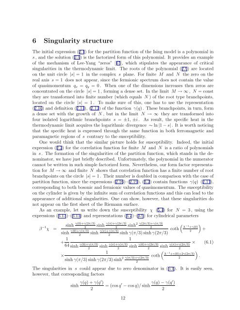
As an example, let us write down the susceptibility χ (5.4) for N = 3 , using the
expressions (3.13)–(3.15) and representations (3.7)–(3.9) for cylindrical parameters
β −1 χ =
sinh γ(0)+γ(2π/3) sinh γ(π)+γ(2π/3) sinh 2 γ(2π/3)+γ(π/3) ( )
2 2 2
sinh γ(0)+γ(π/3) sinh γ(π)+γ(π/3) sinh γ(π/3) sinhγ(2π/3) coth Λ −1 +γ(0)
+
2
2 2
+ 1 1
× (6.1)
64 sinh γ(0)+γ(π/3) sinh γ(π)+γ(π/3) sinh γ(0)+γ(2π/3) sinh γ(π)+γ(2π/3)
2 2 2 2
1
×
sinh γ(π/3) sinhγ(2π/3) sinh 2 γ(π/3)+γ(2π/3)
2
coth
(
Λ −1 +γ(0)+2γ(2π/3)
The singularities in s could appear due to zero denominator in (6.1). It is easily seen,
however, that corresponding factors
sinh γ(q) + γ(q′ )
2
= (cos q ′ − cos q)/ sinh γ(q) − γ(q′ )
2
12
2
)
.