Fractional reaction-diffusion equation for species ... - ResearchGate
Fractional reaction-diffusion equation for species ... - ResearchGate
Fractional reaction-diffusion equation for species ... - ResearchGate
Create successful ePaper yourself
Turn your PDF publications into a flip-book with our unique Google optimized e-Paper software.
<strong>Fractional</strong> <strong>reaction</strong>-<strong>diffusion</strong> <strong>equation</strong> 13<br />
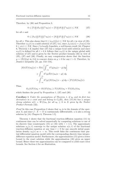
There<strong>for</strong>e, by (36) and Proposition 3,<br />
<strong>for</strong> all x and<br />
0 ≤ [T ( t n )S N ( t n )]n u 0 (x) = [T ( t n )S( t n )]n u 0 (x) ≤ NK (37)<br />
0 ≤ [S N ( t n )T ( t n )]n u 0 (x) = [S( t n )T ( t n )]n u 0 (x) ≤ NK (38)<br />
<strong>for</strong> all x. This also shows that 0 ≤ [u N (t)](x) ≤ NK <strong>for</strong> all x in view of (35).<br />
There<strong>for</strong>e u N (t) is a mild solution of (27), too, since f N (u(x)) = f(u(x)) <strong>for</strong><br />
0 ≤ u(x) ≤ NK. Since f is locally Lipschitz, a well known result [44, Chapter<br />
6, Theorem 1.4] implies that (27) has a unique local mild solution and since<br />
u N (t) is defined <strong>for</strong> all t > 0 it follows that u N (t) is the unique global mild<br />
solution of (27) and is given by the Trotter product <strong>for</strong>mula (32) in view of<br />
(35), (37) and (38). Finally, an easy computation shows that the function<br />
y ↦→ [ ˜S(t)](y) in (14) is concave down on y > 0 <strong>for</strong> any t > 0. There<strong>for</strong>e, by<br />
Jensen’s inequality [21, pp. 153–154],<br />
[∫ ∞<br />
]<br />
[S(t)T (t)u 0 ](x) = ˜S(t) k t (y)u 0 (x − y) dy<br />
−∞<br />
Thus,<br />
≥<br />
=<br />
∫ ∞<br />
−∞<br />
∫ ∞<br />
−∞<br />
k t (y) ˜S(t) [u 0 (x − y)] dy<br />
k t (y) [S(t)u 0 ] (x − y) dy = [T (t)S(t)u 0 ](x).<br />
S N (t)T (t)u 0 = S(t)T (t)u 0 ≥ T (t)S(t)u 0 = T (t)S N (t)u 0<br />
which finishes the proof by Proposition 1, (37) and (38).<br />
Corollary 1 Under the assumptions of Theorem 1, if u 0 and its first two<br />
derivatives in x exist and and belong to C 0 (R), then (27,28) has a unique<br />
strong solution u(t) = W (t)u 0 <strong>for</strong> all u 0 ≥ 0 in X given by the Trotter<br />
Product Formula (32).<br />
Proof In this case Proposition 2 shows that u 0 is in the domain of the operator<br />
A, and since f : X → X is continuously differentiable, u is also a strong<br />
solution by [44, Chapter 6, Theorem 1.5].<br />
⊓⊔<br />
Theorem 1 shows that the fractional <strong>reaction</strong>-<strong>diffusion</strong> <strong>equation</strong> (11) in<br />
continuous time can be solved numerically by computing solutions to one of<br />
its discrete time counterparts (15) or (16) with τ = t/n. The approximate<br />
solutions u n (x, t) converge to the unique solution u(x, t) of the fractional<br />
<strong>reaction</strong>-<strong>diffusion</strong> <strong>equation</strong> at any time t > 0 <strong>for</strong> any smooth initial population<br />
density u 0 (x) as n → ∞. This result links the continuous time partial<br />
differential <strong>equation</strong> model with the corresponding discrete time integrodifference<br />
<strong>equation</strong> model. Furthermore, the approximation (15) gives a lower<br />
bound to the exact solution while the approximation (16) gives an upper<br />
bound. Hence these two approximation can be compared to yield exact error<br />
bounds. See Section 4 <strong>for</strong> an illustration.<br />
⊓⊔


