Fractional reaction-diffusion equation for species ... - ResearchGate
Fractional reaction-diffusion equation for species ... - ResearchGate
Fractional reaction-diffusion equation for species ... - ResearchGate

Create successful ePaper yourself
Turn your PDF publications into a flip-book with our unique Google optimized e-Paper software.
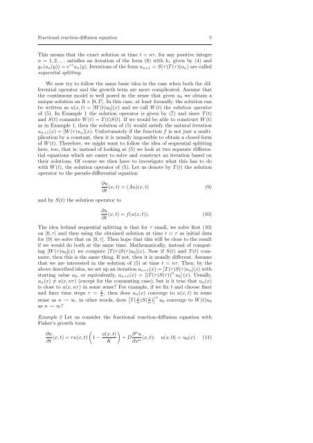
<strong>Fractional</strong> <strong>reaction</strong>-<strong>diffusion</strong> <strong>equation</strong> 5<br />
This means that the exact solution at time t = nτ, <strong>for</strong> any positive integer<br />
n = 1, 2, . . . satisfies an iteration of the <strong>for</strong>m (6) with k τ given by (4) and<br />
g τ (u n (y)) = e rτ u n (y). Iterations of the <strong>for</strong>m u n+1 = S(τ)T (τ)(u n ) are called<br />
sequential splitting.<br />
We now try to follow the same basic idea in the case when both the differential<br />
operator and the growth term are more complicated. Assume that<br />
the continuous model is well posed in the sense that given u 0 we obtain a<br />
unique solution on R × [0, T ]. In this case, at least <strong>for</strong>mally, the solution can<br />
be written as u(x, t) = [W (t)u 0 ](x) and we call W (t) the solution operator<br />
of (5). In Example 1 the solution operator is given by (7) and since T (t)<br />
and S(t) commute W (t) = T (t)S(t). If we would be able to construct W (t)<br />
as in Example 1, then the solution of (5) would satisfy the natural iteration<br />
u n+1 (x) = [W (τ)u n ](x). Un<strong>for</strong>tunately if the function f is not just a multiplication<br />
by a constant, then it is usually impossible to obtain a closed <strong>for</strong>m<br />
of W (t). There<strong>for</strong>e, we might want to follow the idea of sequential splitting<br />
here, too, that is; instead of looking at (5) we look at two separate differential<br />
<strong>equation</strong>s which are easier to solve and construct an iteration based on<br />
their solutions. Of course we then have to investigate what this has to do<br />
with W (t), the solution operator of (5). Let us denote by T (t) the solution<br />
operator to the pseudo-differential <strong>equation</strong><br />
and by S(t) the solution operator to<br />
∂u<br />
(x, t) = (Au)(x, t) (9)<br />
∂t<br />
∂u<br />
(x, t) = f(u(x, t)). (10)<br />
∂t<br />
The idea behind sequential splitting is that <strong>for</strong> τ small, we solve first (10)<br />
on [0, τ] and then using the obtained solution at time t = τ as initial data<br />
<strong>for</strong> (9) we solve that on [0, τ]. Then hope that this will be close to the result<br />
if we would do both at the same time. Mathematically, instead of computing<br />
[W (τ)u 0 ](x) we compute [T (τ)S(τ)u 0 ](x). Now if S(t) and T (t) commute,<br />
then this is the same thing. If not, then it is usually different. Assume<br />
that we are interested in the solution of (5) at time t = nτ. Then, by the<br />
above described idea, we set up an iteration u n+1 (x) = [T (τ)S(τ)u n ](x) with<br />
starting value u 0 , or equivalently, u n+1 (x) = [(T (τ)S(τ)) n u 0 ] (x). Usually,<br />
u n (x) ≠ u(x, nτ) (except <strong>for</strong> the commuting case), but is it true that u n (x)<br />
is close to u(x, nτ) in some sense For example, if we fix t and choose finer<br />
and finer time steps τ = t n , then does u n(x) converge to u(x, t) in some<br />
sense as n → ∞, in other words, does [ T ( t n )S( t n )] n<br />
u0 converge to W (t)u 0<br />
as n → ∞<br />
Example 2 Let us consider the fractional <strong>reaction</strong>-<strong>diffusion</strong> <strong>equation</strong> with<br />
Fisher’s growth term<br />
( )<br />
∂u<br />
∂t (x, t) = ru(x, t) u(x, t)<br />
1 − + D ∂α u<br />
K ∂x α (x, t); u(x, 0) = u 0(x) (11)