Fractional reaction-diffusion equation for species ... - ResearchGate

More documents

Recommendations

Info

16 Baeumer, Kovács, Meerschaert 0 < α < 1 the last term in the integral (26) converges, and hence we can choose a so that Au(x) = ∫ ∞ 0 u(x − y) − u(x) y Cy −α dy. (39) Then we see that the fractional derivative is a weighted average of difference quotients, with power law weights deriving from the underlying jump intensity. Using the fractional derivative generator in the abstract reactiondiffusion equation (5) corresponds to an α-stable dispersal kernel in the corresponding discrete-time integro-difference equation (6). Along with the Gaussian kernel (the special case α = 2), these dispersal kernels are distinguished by the stability property: k t (y) = t −1/α k(yt −1/α ) for all y ∈ R and all t > 0. Hence they are strongly indicated when the shape of the dispersal kernel is time-independent. Furthermore, since they derive from central limit theorems, they are in some sense universal. Finally, although these α- stable probability density functions cannot usually be written in closed form, probabilists have developed fast numerical methods for computing them [42]. Combining this with Theorem 1 allows the efficient solution of the fractional reaction-diffusion equation, as well as monotone error bounds. We will illustrate the application of these methods in the next section. Remark 4 A wide variety of alternative models can be obtained by considering different infinitely divisible densities k as the dispersal kernel. The infinitely divisible densities are convenient because one can define the integrodifference equation (6) at any time scale τ based on the convolution power k τ . The results of this paper also yield the corresponding reaction-diffusion model with a diffusion operator A exhibiting as the generator of the corresponding infinitely divisible semigroup. Lockwood et al. [30] employ a Laplace (double exponential), or more generally, a double Gamma family of dispersion kernels, which are infinitely divisible with Lévy representation [ta, 0, tφ] with jump intensity φ(y) = |y| −1 e −c|y| . In this case the last term in the integral (26) converges, and hence we can choose a so that Au(x) = ∫ ∞ −∞ u(x − y) − u(x) |y| e −c|y| dy (40) an exponentially weighted derivative, which is similar to the fractional derivative formula (39) but with different weights [29]. For an exponential or Gamma dispersal kernel, the generator formula is the same as (40) except that the integral is taken over y > 0. Clarke et al. [16,17] employ the Student-t dispersal kernel, which is infinitely divisible with Lévy representation as specified in [23, Remark 2.3] in terms of Bessel functions. Substituting into (26) yields the corresponding generator, connecting the integro-difference equation (6) with a Student-t dispersal kernel to the analogous reaction-diffusion equation (5).
Fractional reaction-diffusion equation 17 4 Numerical Experiments Consider a fractional reaction-diffusion equation using Fisher’s growth equation and a symmetric (Riesz) fractional diffusion term of order 1 < α ≤ 2: ( ) ∂u ∂t (x, t) = D ∂α u ∂|x| α (x, t) + ru(x, t) u(x, t) 1 − , u(x, 0) = u 0 (x). (41) K Solutions to this equation can be computed using the results of Theorem 1, using the integro-difference model (6) as an approximation where the dispersal kernel k τ (y) is the symmetric α-stable probability density function whose Fourier transform is e −Dτ|λ|α for some D > 0. 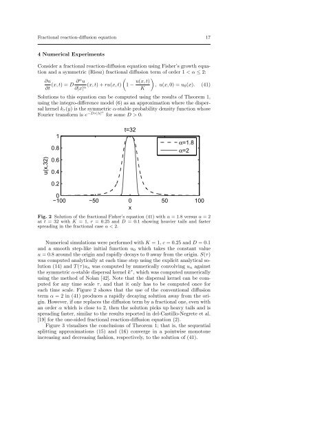u(x,32) 1 0.8 0.6 0.4 0.2 t=32 α=1.8 α=2 0 −100 −50 0 50 100 x Fig. 2 Solution of the fractional Fisher’s equation (41) with α = 1.8 versus α = 2 at t = 32 with K = 1, r = 0.25 and D = 0.1 showing heavier tails and faster spreading in the fractional case α < 2. Numerical simulations were performed with K = 1, c = 0.25 and D = 0.1 and a smooth step-like initial function u 0 which takes the constant value u = 0.8 around the origin and rapidly decays to 0 away from the origin. S(τ) was computed analytically at each time step using the explicit analytical solution (14) and T (τ)u n was computed by numerically convolving u n against the symmetric α-stable dispersal kernel k τ , which was computed numerically using the method of Nolan [42]. Note that the dispersal kernel can be computed for any time scale τ, and that it only has to be computed once for each time scale. Figure 2 shows that the use of the conventional diffusion term α = 2 in (41) produces a rapidly decaying solution away from the origin. However, if one replaces the diffusion term by a fractional one, even with an order α which is close to 2, then the solution picks up heavy tails and is spreading faster, similar to the results reported in del-Castillo-Negrete et al. [19] for the one-sided fractional reaction-diffusion equation (2). Figure 3 visualises the conclusions of Theorem 1; that is, the sequential splitting approximations (15) and (16) converge in a pointwise monotone increasing and decreasing fashion, respectively, to the solution of (41).
Page 1 and 2: Noname manuscript No. (will be inse
Page 3 and 4: Fractional reaction-diffusion equat
Page 15: Fractional reaction-diffusion equat
Page 21: Fractional reaction-diffusion equat

Fractional reaction-diffusion equation for species ... - ResearchGate

Create successful ePaper yourself

Delete template?

Save as template?