Albrecht 19.pdf - Marriott School
Albrecht 19.pdf - Marriott School
Albrecht 19.pdf - Marriott School

Create successful ePaper yourself
Turn your PDF publications into a flip-book with our unique Google optimized e-Paper software.
76154_23_ch19_p942-1006.qxd 3/1/07 3:35 PM Page 942<br />
19<br />
C H A P T E R<br />
© AP PHOTO/ROBERT F BUKATY<br />
Controlling Cost,<br />
Profit, and Investment<br />
Centers
76154_23_ch19_p942-1006.qxd 3/1/07 3:35 PM Page 943<br />
LEARNING OBJECTIVES<br />
After studying this chapter, you should be able to:<br />
1<br />
2<br />
3<br />
Describe the responsibility accounting concept<br />
and identify the three types of organizational<br />
control units. The idea behind<br />
responsibility accounting is that the performance of<br />
a manager should be based only on those items<br />
(costs, revenues, or assets) over which that manager<br />
exercises some control.<br />
Describe standard costing and use materials<br />
and labor cost variance analysis to explain<br />
how performance is controlled in<br />
cost centers. In order to evaluate the performance<br />
of a manager, there must be a standard to<br />
which the performance of the manager can be<br />
compared. In a cost center, where the manager has<br />
control only over the costs, the actual amount paid<br />
for and used in materials and labor is compared to<br />
the amount that should have been paid for and<br />
used; any difference is called a cost variance.<br />
Use segment margin statements and<br />
revenue variance analysis to explain how<br />
performance is controlled in profit<br />
centers. Manager performance in profit centers<br />
should be evaluated solely on expenses and<br />
revenues that are directly related to that business<br />
segment. Revenue variances can be combined with<br />
cost variances to control and evaluate performance<br />
in profit centers.<br />
4<br />
5<br />
6<br />
Use ROI and residual income analysis to<br />
explain how performance is controlled<br />
in investment centers. A manager of an investment<br />
center has responsibility to effectively<br />
manage costs, revenues, and assets. Computation<br />
of return on investment (ROI) and residual income<br />
incorporates cost, revenue, and asset performance.<br />
EXPANDED<br />
material<br />
Compute and interpret variable overhead<br />
cost variances. In addition to managing the<br />
cost of materials and labor, the manager of a cost<br />
center is also responsible for managing variable<br />
manufacturing overhead costs. The actual variable<br />
overhead cost incurred is compared to the cost<br />
that should have been incurred given the level<br />
of activity.<br />
Compute and interpret fixed overhead<br />
cost variances. Many cost center managers are<br />
responsible for fixed manufacturing overhead costs.<br />
Fixed overhead variances occur both because of a<br />
difference between actual and budgeted spending<br />
and because of a difference between the actual<br />
and budgeted levels of activity.
76154_23_ch19_p942-1006.qxd 3/1/07 3:35 PM Page 944<br />
944 Part 6 Control in a Management Accounting System<br />
S E T T I N G T H<br />
S E T T I N G T H<br />
E E G G A A T T S S E E<br />
Before Randy Curran was appointed CEO, ICG<br />
Communications was losing $34 million a<br />
month. That was in September 2000. On<br />
November 14, 2000, ICG filed for Chapter 11<br />
bankruptcy. BusinessWeek reported that ICG’s<br />
survival was unlikely. However, ICG recovered<br />
from hard times to become a smaller but prosperous<br />
company and was finally purchased<br />
by Level 3 Communications in 2006 for<br />
$163 million. ICG’s story is about how a company<br />
gone awry can be saved through fiscal responsibility<br />
and good management control. 1<br />
ICG provides voice, data, and Internet communications<br />
services in targeted cities. During<br />
the heyday of the Internet explosion in the late<br />
1990s, ICG became the poster child for the<br />
failed “build it and they will come” business<br />
model. During this time, ICG quickly burned<br />
through $2 billion raised through Wall Street<br />
investors. Randy Curran, the current CEO, is<br />
largely responsible for recovering ICG after the<br />
previous CEO went on a spending spree hosting<br />
elaborate parties and building excessive<br />
facilities in an apparent effort to put himself and<br />
his company in the spotlight of trade and<br />
business publications and the society pages.<br />
Randy Curran faced a difficult task in carefully<br />
controlling a turnaround of ICG’s financial position.<br />
A high level view of the company revealed<br />
numerous problems that needed immediate attention.<br />
Curran realized that a poor-performing<br />
network would kill the business, regardless of<br />
the impressive size and scale of the network<br />
operation. He identified a large number of unprofitable<br />
products, services, and customers.<br />
ICG emerged from Chapter 11 protection<br />
on October 10, 2002, after its employee head<br />
count had dropped from 3,000 to 1,000. Randy<br />
Curran and his management team had to carefully<br />
refocus the company on controlling costs,<br />
managing revenues, and effectively using its assets.<br />
It took a lot of work to bring ICG through<br />
the next three and half years to eventually negotiate<br />
a successful acquisition. Companies<br />
such as ICG provide good outlines for other<br />
tech companies on how to control and manage<br />
a successful (sometimes smaller) business in<br />
the post-Internet bubble era.<br />
In Chapter 18, we created the master budget,<br />
which is a major planning tool for management.<br />
In this chapter, we will examine how<br />
managers create and maintain an effective system<br />
of control within their organizations. Traditional<br />
control systems are initially based on using the<br />
standard cost and revenue data created in the<br />
master budget. These data are used to assess<br />
business processes throughout the year in order<br />
to identify performance in various organization<br />
units that require management attention.<br />
In the process of establishing effective management<br />
control within an organization, it is critical<br />
to clearly define each division’s and each<br />
person’s specific responsibility within the organization.<br />
Because it is often difficult to separate the<br />
performance of a unit from the performance of its<br />
managers, managers are most often evaluated on<br />
how well their units perform. If managers are<br />
responsible for costs only, they are usually evaluated<br />
on how well they control costs. If they are<br />
responsible for revenues and costs, they are usually<br />
evaluated on the profitability of their units.<br />
And, if they are responsible for costs, revenues,<br />
and investments, managers are most frequently<br />
evaluated on the return their division investments<br />
generate. In the case of ICG, the new CEO was responsible<br />
for doing a better job than had the previous<br />
CEO of controlling costs, revenues, and<br />
investments. Because the company initially lost<br />
large sums of money, one may fairly question the<br />
effectiveness of cost, revenue, and asset controls<br />
at ICG prior to 2000. On the other hand, ICG’s<br />
turnaround since 2000 is largely attributable to<br />
Randy Curran’s fiscal responsibility and his efforts<br />
to bring ICG’s operations under control.<br />
1 Paul M. Sherer and Gary McWilliams, “How a Brash Provider of Internet Services Became Unplugged,” The Wall Street Journal,<br />
November 13, 2000, p. A1; Paul M. Sherer, “ICG Files for Protection from Creditors,” The Wall Street Journal, November 15,<br />
2000, p. A1; Peter Elstrom, “Dead Companies Walking,” BusinessWeek Online, January 22, 2001; John Sullivan and Tom Cross,<br />
“A New Day at ICG,” Boardwatch Magazine, April 2002, Vol. 16, Issue 4, pp. 42–44; “ICG out of Bankruptcy,” Denver<br />
Business Journal, October 10, 2002, http://denver.bizjournals.com, accessed September 5, 2003; Client Interview with<br />
ICG, http://www.gapinter.com/ClientProfiles, accessed September 5, 2003. Level 3 Communications, Inc. news release,<br />
May 31, 2006.
76154_23_ch19_p942-1006.qxd 3/1/07 3:35 PM Page 945<br />
Controlling Cost, Profit, and Investment Centers Chapter 19 945<br />
Describe the<br />
responsibility<br />
accounting concept<br />
and identify the<br />
three types of<br />
organizational<br />
control units.<br />
segments<br />
Parts of an organization<br />
requiring separate reports<br />
for evaluation by<br />
management.<br />
1<br />
Control of Divisions and Personnel<br />
in Different Types of Operating Units<br />
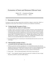
Most companies are made up of a number of relatively independent segments<br />
or subunits, sometimes called groups, divisions, or subsidiaries. As an example,<br />
Exhibit 1 shows an organizational chart for a hypothetical company that we will<br />
call International Manufacturing Corporation (IMC). IMC has three operating<br />
(subsidiary) companies: Acme Computer, Edison Automobile, and Jennifer<br />
Cosmetics. Although each of these companies has several divisions and other subsegments,<br />
only a few of those for Edison Automobile are shown. Edison has three<br />
geographic bases: the United States, the Far East, and Europe. The making and selling<br />
of automobiles in the Far East division is further broken down into the Japan<br />
and Korea units. The Japan unit is separated into its sales, manufacturing, and<br />
service functions. Edison Automobile’s other geographic divisions have similar<br />
subsegments.<br />
EXHIBIT 1<br />
An Organizational Chart<br />
International<br />
Manufacturing<br />
Corporation (IMC)<br />
Acme<br />
Computer<br />
Company<br />
Edison<br />
Automobile<br />
Company<br />
Jennifer<br />
Cosmetics<br />
Company<br />
U.S.<br />
Operations<br />
Far East<br />
Operations<br />
Europe<br />
Operations<br />
Japan<br />
Operations<br />
Korea<br />
Operations<br />
Sales<br />
Manufacturing<br />
Service
76154_23_ch19_p942-1006.qxd 3/1/07 3:35 PM Page 946<br />
946 Part 6 Control in a Management Accounting System<br />
operating capital<br />
Funds available for use in<br />
financing the day-to-day<br />
activities of a business.<br />
decentralized<br />
company<br />
An organization in which<br />
managers at all levels<br />
have the authority to make<br />
decisions concerning the<br />
operations for which they<br />
are responsible.<br />
You will notice that IMC uses different criteria to define its segments at each level.<br />
At the highest level, product group (computers, autos, cosmetics) is used, probably because<br />
there is a significant difference in the business knowledge needed to produce and<br />
sell these products. At the middle level, segments are defined geographically because of<br />
the unique needs of each market and the distances involved. At the lowest level, each<br />
country unit is subdivided by business function—sales, manufacturing, and service.<br />
Given the organizational chart in Exhibit 1, how much autonomy should the executives<br />
of each division be granted by corporate management If each company (Acme,<br />
Edison, and Jennifer) has its own president, vice presidents, and other officers, should<br />
these executives be allowed to operate independently of one another If Acme,<br />
for example, is the most profitable company, should it be given more operating<br />
capital than Edison and Jennifer, or less Should a decision for Acme to expand<br />
into hand-held computers be made by Acme’s executives or by IMC’s corporate<br />
officers Within Edison Automobile, how much autonomy should each of the geographic<br />
offices have Should a decision to double the advertising budget or offer<br />
consumer rebates in the Far East operations be made by the manager of that division, by<br />
the president of Edison Automobile, or by the CEO of IMC<br />
These are challenging questions. In fact, it would probably be difficult to find two companies<br />
that would answer them the same way. Assuming that IMC is basically a decentralized<br />
company, managers at all levels will have the authority to make<br />
decisions concerning the operations for which they are directly responsible.<br />
Regarding the question of rebates in the Far East, for example, the operating manager<br />
of that geographic division should probably decide whether to offer them.<br />
Likewise, the manager of the Japan Manufacturing division should decide where to<br />
buy engine parts, and the manager of the Service division should have primary responsibility<br />
for setting the price to charge for repairing a muffler in Japan. These<br />
managers should also be held responsible for the consequences of their decisions.<br />
Benefits and Problems of Decentralization<br />
centralized company<br />
To what degree should a company decentralize Clearly, a large company<br />
An organization in which<br />
employing thousands of people in different geographic areas could not remain<br />
top management makes<br />
completely centralized, with top management making all the decisions. The president<br />
of IMC would not know enough about the costs and varieties of paint in<br />
most of the major<br />
decisions for the entire<br />
Japan, for example, or have enough time to make all the operating decisions for<br />
company rather than<br />
the manufacturing subsegment of the Japan operations of Edison Automobile.<br />
delegating decisions to<br />
Though such decisions would never be made strictly by the president of a large<br />
managers at lower levels.<br />
international company, they would be made at a higher level in a centralized<br />
company than in a decentralized one.<br />
Currently, the trend in most companies is to decentralize. The reasons often cited for<br />
making decisions at the lowest possible level in an organization are:<br />
1. Segment managers usually have more information about matters within their area of<br />
responsibility than do managers at higher levels.<br />
2. Segment managers are in a better position to see current problems and to react<br />
quickly to local situations.<br />
3. Higher-level management can spend more time on broader policy and strategic issues<br />
because the burden of daily decision making is distributed.<br />
4. Segment managers have a greater incentive to perform well because they receive<br />
the credit (or blame) for performance resulting from their decisions.<br />
5. Employees have greater incentives and motivation to perform well because there<br />
are more opportunities for advancement into leadership positions when a company<br />
is decentralized.<br />
6. Managers and officers can be evaluated more easily because their responsibilities are<br />
more clearly defined.
76154_23_ch19_p942-1006.qxd 3/1/07 3:35 PM Page 947<br />
Controlling Cost, Profit, and Investment Centers Chapter 19 947<br />
goal congruence<br />
The selection of goals for<br />
responsibility centers that<br />
are consistent, or congruent,<br />
with those of the<br />
company as a whole.<br />
Decentralization has its drawbacks as well. Decisions made by managers of decentralized<br />
units are sometimes not consistent with the overall objectives of the firm. For example,<br />
Edison Automobile might find it less expensive to buy computer parts for its automobiles<br />
from an outside source than from Acme Computer, or the Service division of Japan operations<br />
may find it cheaper to buy repair parts from outsiders rather than from the Manufacturing<br />
division. Such decisions would allow the buying divisions to report lower costs, but the decisions<br />
might decrease the company’s overall profitability (depending on whether or not<br />
costs in other division can actually be avoided when Edison Automobile decides to purchase<br />
computer parts from an outside vendor).<br />
There are two ways to prevent such problems. First, certain decisions should<br />
be centralized. For example, all decisions related to insurance coverage, which<br />
benefits the entire company, should probably be made at the corporate level.<br />
Second, an effective system of responsibility accounting should be established so<br />
that a manager’s decisions will benefit not only the segment but also the firm as<br />
a whole. This goal congruence, whereby the goals of the company and all its<br />
segments are in harmony, can be achieved only if the responsibility accounting<br />
system is well designed.<br />
responsibility<br />
accounting<br />
A system of evaluating performance;<br />
managers are<br />
held accountable for the<br />
costs, revenues, assets, or<br />
other elements over which<br />
they have control.<br />
exception reports<br />
Reports that highlight variances<br />
from, or exceptions<br />
to, the budget.<br />
Responsibility Accounting<br />
Responsibility accounting is a system in which managers are assigned and held<br />
accountable for certain costs, revenues, and/or assets. There are two important<br />
behavioral considerations in assigning responsibilities to managers.<br />
• First, the responsible manager should be involved in developing the plan<br />
for the unit over which the manager has control. Current research indicates<br />
that people are more motivated to achieve a goal if they participate in setting<br />
it. Such participation assures that the goals will be reasonable and, perhaps<br />
more importantly, that they will be perceived to be reasonable by the<br />
managers.<br />
• Second, a manager should be held accountable only for those costs,<br />
revenues, or assets over which the manager has substantial control. Some<br />
costs may be generated within a segment, but control over them lies outside<br />
that unit. The manager of the Japan Manufacturing division, for example,<br />
may be held responsible for labor costs, but employee wages may be determined<br />
by a union scale controlled elsewhere. Admittedly, determining “substantial<br />
control” requires a judgment based on the circumstances, but if all<br />
relevant factors are considered, careful and fair judgments can be made.<br />
Responsibility Accounting Reports Regardless of the degree of autonomy given to<br />
managers at various operating levels, performance reports based on responsibility accounting<br />
are needed at all levels of the organization. At the lowest levels, these reports tell managers<br />
where corrective action must be taken to control their segments’ operations. At top<br />
levels, these reports keep management informed of the activities of all segments. The reports<br />
are then used to reward past performance and set incentives for future performance.<br />
Exhibit 2 illustrates the kind of responsibility accounting reports a company might<br />
use. Note that reporting begins at the bottom and “rolls” upward, with each manager receiving<br />
information on the operations for which that manager is responsible, as well as<br />
summary information on the performance of lower-level managers. Note also that<br />
these reports are exception reports, meaning that variances from, or exceptions<br />
to, the budget are highlighted. In the report, unfavorable variances are<br />
labeled “U” while favorable variances are labeled “F.” Such reports direct management<br />
immediately to the areas requiring their attention. Note that Exhibit 2<br />
reports only on cost management. In this chapter, we’ll also discuss reporting<br />
performance on revenue and asset management.
76154_23_ch19_p942-1006.qxd 3/1/07 3:35 PM Page 948<br />
948 Part 6 Control in a Management Accounting System<br />
EXHIBIT 2<br />
Responsibility Accounting Reports for Edison Automobile<br />
Company of IMC (in thousands of dollars)<br />
Budgeted Actual<br />
President, Edison Automobile Responsibility Centers Costs Costs Variance*<br />
The president receives from each General Administration . . . . . . . . . $ 89,000 $ 81,000 $ 8,000 F<br />
geographic area of operations a report United States . . . . . . . . . . . . . . . . 145,000 151,000 6,000 U<br />
summarizing its performance. The Far East . . . . . . . . . . . . . . . . . . . . 58,000 65,000 7,000 U<br />
president can see where further Europe . . . . . . . . . . . . . . . . . . . . . 111,000 99,000 12,000 F<br />
investigation needs to be done by Total costs . . . . . . . . . . . . . . . . . $403,000 $396,000 $ 7,000 F<br />
tracing the differences between budget<br />
and actual downward to their sources.<br />
Budgeted Actual<br />
Far East Operations Responsibility Centers Costs Costs Variance<br />
The manager of Far East operations Japan Operations . . . . . . . . . . . . . $ 21,000 $ 23,000 $ 2,000 U<br />
receives a report from each country Korea Operations . . . . . . . . . . . . . 18,000 17,000 1,000 F<br />
segment’s head. These reports are China Operations . . . . . . . . . . . . . 11,000 13,000 2,000 U<br />
then summarized and passed on to the Thailand Operations . . . . . . . . . . . 8,000 12,000 4,000 U<br />
president of Edison Automobile.<br />
Total costs . . . . . . . . . . . . . . . . . $ 58,000 $ 65,000 $ 7,000 U<br />
Budgeted Actual<br />
Japan Operations Responsibility Centers Costs Costs Variance<br />
The manager of Japan operations Sales . . . . . . . . . . . . . . . . . . . . . . $ 2,800 $ 1,700 $ 1,100 F<br />
receives from each unit a report Manufacturing . . . . . . . . . . . . . . . . 9,000 10,200 1,200 U<br />
summarizing its performance. These Service . . . . . . . . . . . . . . . . . . . . . 5,800 6,500 700 U<br />
reports are combined and sent up to Administration . . . . . . . . . . . . . . . . 3,400 4,600 1,200 U<br />
the next level, the manager of Total costs . . . . . . . . . . . . . . . . . $ 21,000 $ 23,000 $ 2,000 U<br />
Far East operations.<br />
Variable Costs Budgeted Actual<br />
Japan Manufacturing Division of Manufacturing Costs Costs Variance<br />
The Manufacturing division supervisor Direct materials . . . . . . . . . . . . . . . $ 2,000 $ 2,500 $ 500 U<br />
receives a performance report on the Direct labor . . . . . . . . . . . . . . . . . . 6,000 6,400 400 U<br />
supervisor’s center of responsibility. Manufacturing overhead . . . . . . . . 1,000 1,300 300 U<br />
The totals from these reports are then Total costs . . . . . . . . . . . . . . . . . $ 9,000 $ 10,200 $ 1,200 U<br />
communicated to the manager of<br />
Japan operations, the next level<br />
of responsibility.<br />
*U means unfavorable.<br />
responsibility center<br />
An organizational unit in<br />
which a manager has<br />
control over and is held<br />
accountable for<br />
performance.<br />
cost center<br />
An organizational unit in<br />
which a manager has<br />
control over and is held<br />
accountable for cost<br />
performance.<br />
Responsibility Centers In our example, the president of IMC is responsible<br />
for the entire organization and should be held accountable for the company’s<br />
overall successes and failures. At lower levels, the president of Edison Automobile<br />
Company, the manager of Edison’s operations in the Far East, the manager in<br />
charge of Japan operations in Edison’s Far East operations, and the manager of the<br />
Japan Manufacturing division, for example, would be held responsible for operations<br />
within their respective units.<br />
Each unit is referred to as a responsibility center, and, depending on the<br />
operation, it may be a cost, profit, or investment center. As the name implies,<br />
a cost center is any organizational unit in which the manager of that unit has<br />
control only over the costs incurred. The manager of a cost center has no responsibility<br />
for revenues or assets, either because revenues are not generated in
76154_23_ch19_p942-1006.qxd 3/1/07 3:35 PM Page 949<br />
Controlling Cost, Profit, and Investment Centers Chapter 19 949<br />
profit center<br />
An organizational unit in<br />
which a manager has<br />
control over and is held<br />
accountable for both cost<br />
and revenue performance.<br />
investment center<br />
An organizational unit in<br />
which a manager has<br />
control over and is held<br />
accountable for cost,<br />
revenue, and asset<br />
performance.<br />
the center or because revenues and assets are under the control of someone else.<br />
The manufacturing unit of Japan operations of IMC, for example, could be designated<br />
a cost center. A profit center manager, however, has responsibility for<br />
both costs and revenues. Profit centers are usually found at higher levels in an<br />
organization than are cost centers. The geographic regions (United States, Far<br />
East, and Europe, as well as various country operations within the Far East region)<br />
of Edison Automobile could be profit centers (though they could also be<br />
designated as investment centers).<br />
In an investment center, the manager is responsible for costs, revenues, and<br />
assets. This means that the manager is responsible not only for operating costs and<br />
revenues, but also for determining the amount of funds to be invested in the center’s<br />
plant and equipment and for the rate of return earned on those investments.<br />
Investment centers are usually found at relatively high levels in organizations. The<br />
different companies in IMC (Acme Computer, Edison Automobile, and Jennifer<br />
Cosmetics) would probably be investment centers.<br />
R E M E M B E R T H I S . . .<br />
• Decentralized companies delegate decisions and responsibility<br />
to lower-level managers, while centralized companies retain<br />
decisions and responsibility to run the business at higher levels of<br />
management.<br />
• In order for managers to operate effectively in decentralized<br />
companies, a system of responsibility accounting should be<br />
established.<br />
• Responsibility accounting is based on carefully identifying business<br />
units in the organization and classifying those business units as:<br />
• cost centers,<br />
• profit centers, or<br />
• investment centers.<br />
• Generally, cost centers are found at lower levels of the organization,<br />
while profit and investment centers are found at higher levels of<br />
the organization.<br />
Describe standard<br />
costing and use materials<br />
and labor cost<br />
variance analysis to<br />
explain how performance<br />
is controlled<br />
in cost centers.<br />
2<br />
Standard Cost Systems<br />
If managers are to be held responsible for the costs incurred in their centers,<br />
they must have control over those costs, have relevant information about those<br />
costs, and have a system that focuses on and supports effective cost controls.<br />
Traditionally, companies have used a standard costing system that isolates differences<br />
between actual and standard (or budgeted) costs to determine whether<br />
costs are too high or too low, as well as whether costs are improving (decreasing)<br />
or getting worse (increasing). This is critical information if the organization<br />
expects to be competitive. In a standard cost management system, standard costs<br />
are compared to actual costs, and variances are computed.<br />
Service, merchandising, and manufacturing firms that use standard costing will design<br />
their accounting systems to incorporate standard costs and variances. This type of<br />
system, called a standard cost system, is a cost-accumulation process based on costs that<br />
should have been incurred rather than costs that were actually incurred (see page 950 for<br />
definition). The steps in establishing and operating a standard cost system are:
76154_23_ch19_p942-1006.qxd 3/1/07 3:35 PM Page 950<br />
950 Part 6 Control in a Management Accounting System<br />
Step<br />
1Develop<br />
standard<br />
costs.<br />
Step<br />
2Collect<br />
actual<br />
costs.<br />
Step<br />
3Compare<br />
actual costs<br />
to standard<br />
costs and<br />
identify<br />
variances.<br />
4Step<br />
Journalize<br />
actual costs<br />
and standard<br />
costs and<br />
record the<br />
variances.<br />
Step<br />
Report 5results<br />
including<br />
variances to<br />
managers<br />
responsible<br />
for variances.<br />
Step<br />
6Analyze<br />
causes of<br />
significant<br />
controllable<br />
variances.<br />
Step<br />
7Take action<br />
to eliminate<br />
variances<br />
or revise<br />
standard<br />
costs.<br />
standard cost system<br />
A cost-accumulation system<br />
in which standard<br />
costs are used as product<br />
costs instead of actual<br />
costs. The standard<br />
costs are then adjusted to<br />
actual costs when financial<br />
reports are created.<br />
This adjustment creates<br />
variances that are reported<br />
to management.<br />
These steps describe a typical standard cost system. You are likely to find an<br />
extensive standard cost system in most manufacturing firms, which usually have<br />
standard costs for direct materials, direct labor, and manufacturing overhead.<br />
However, many service and merchandising firms also use a standard cost system<br />
to effectively manage critical costs in their organizations. Standard costs usually<br />
are often stored in a computer. In Chapter 18 we created an operating budget for<br />
Sunbird Boat Company. A critical part of creating this budget was establishing the<br />
standard costs to produce a 15-foot fishing boat. These costs are reported in<br />
Chapter 18, although they are spread across a number of budget schedules that<br />
we created in that chapter. The management team and accountants at Sunbird<br />
Boat Company can compile all of these standard cost data for 15-foot fishing boats.<br />
The standard costs for Sunbird Boat Company are shown in Exhibit 3. We will use<br />
the data in Exhibit 3 to illustrate how variances are calculated and analyzed.<br />
CAUTION<br />
All of the cost variances we compute in this<br />
chapter are based on Sunbird’s standard cost<br />
card. Be sure to return to Exhibit 3 to review<br />
these standards as you work through the remainder<br />
of this chapter. (Note that these are<br />
the same standard costs and quantities we<br />
used to build budgets for Sunbird Boat<br />
Company in Chapter 18.)<br />
Determining Standard Costs<br />
In a manufacturing firm, standard costs are<br />
determined on the basis of careful analysis<br />
and the experience of many people, including<br />
accountants, industrial engineers, purchasing<br />
agents, and the managers of the<br />
departments to be judged. Accountants play<br />
an important role in developing standard<br />
costs because they have the data needed to<br />
determine how costs have changed in the<br />
past in relation to levels of activity. This is not<br />
an easy task. Changes in methods of production,<br />
technology, worker efficiency, and plant<br />
layout, for example, can affect the behavior<br />
EXHIBIT 3<br />
Standard Cost Card<br />
Sunbird Boat Company<br />
Standard Cost Card—15-Foot Fishing Boats<br />
(1) (2) (3)<br />
Standard Standard Standard<br />
Quantity Price or Rate Cost (1) (2)<br />
Inputs:<br />
Direct materials:<br />
Wood . . . . . . . . . . . . . . . . . . . . . . . . . 100 feet $10.00 $1,000.00<br />
Fiberglass . . . . . . . . . . . . . . . . . . . . . . 40 feet 5.00 200.00<br />
Direct labor . . . . . . . . . . . . . . . . . . . . . . 80 hours 20.00 1,600.00<br />
Manufacturing overhead:<br />
Variable . . . . . . . . . . . . . . . . . . . . . . . . 80 hours 7.50 600.00<br />
Fixed . . . . . . . . . . . . . . . . . . . . . . . . . . 80 hours 20.00 1,600.00<br />
Total standard cost per boat . . . . . . . . . . $5,000.00
76154_23_ch19_p942-1006.qxd 3/1/07 3:35 PM Page 951<br />
Controlling Cost, Profit, and Investment Centers Chapter 19 951<br />
variance<br />
Any deviation from<br />
standard.<br />
management by<br />
exception<br />
The strategy of focusing<br />
attention on significant<br />
deviations from standard<br />
costs or expectations.<br />
of costs. Before using standard costs to create the annual budget, past cost data often have<br />
to be adjusted to take changes in operating conditions into account. These changes sometimes<br />
occur gradually and may not be easily noticeable, making it difficult for accountants to<br />
identify cost characteristics that will be useful in setting standards for the future.<br />
Engineers are often involved in setting standard costs because of their knowledge of<br />
the most efficient way of performing each task in relation to the existing technology of the<br />
operation. Managers who will be judged by the standard costs should be involved in the<br />
standard-setting process; they are more likely to be motivated to meet standards if they<br />
have participated in setting the standards and have accepted them. In addition, managers’<br />
experience and judgment can be quite valuable in establishing appropriate cost standards.<br />
Once management has established a standard price for each resource (direct materials,<br />
direct labor, and manufacturing overhead) and has determined the standard input<br />
quantity allowed, the standard price is multiplied by the standard quantity to arrive at a<br />
S T O P & T H I N K<br />
Is it possible for a company to have positive<br />
variances (actual costs are less than standard<br />
costs) and still have problems Can you think<br />
of an example<br />
standard dollar cost for the product or service. Actual costs are then compared<br />
with these standards to calculate the variance, the amount by which the actual<br />
cost differs from the standard. This variance, if significant, is a signal to management<br />
that costs may be “out of control” and that corrective action should be<br />
taken to eliminate the variance. This process of using variances from a standard<br />
to isolate problem areas is called management by exception and is the basis<br />
for establishing control in a management accounting system.<br />
Let’s review Exhibit 3 again. You can see in the third column that the standard<br />
costs to produce boats at Sunbird Boat Company are composed of both a<br />
price (or rate) for the input and a quantity (or usage) of the input. Hence, comparing<br />
actual costs with standard costs results in two variances: a price (or rate)<br />
variance and a quantity (or usage) variance. These variances are usually computed<br />
for direct materials, direct labor, and variable manufacturing overhead.<br />
We’re going to explain how direct materials<br />
variances are computed and analyzed<br />
by using the Sunbird Boat Company as an<br />
example. Then, we will explain the computation<br />
and analysis of direct labor variances.<br />
The more complex variances for<br />
manufacturing overhead will be discussed<br />
and illustrated in the expanded material<br />
section of this chapter.<br />
Controlling Performance in Cost Centers<br />
You should understand that managers of cost centers are responsible for costs incurred,<br />
and most cost centers usually have one type of cost that is more significant than any other.<br />
In service organizations, salaries are generally the major cost. In wholesale and retail businesses,<br />
the cost of merchandise purchased for resale is often the most significant cost. In<br />
manufacturing firms, costs incurred to make products (direct materials, direct labor,<br />
and manufacturing overhead) are usually most significant. The standard cost system we’re<br />
presenting here is an effective method of controlling these kinds of costs.<br />
Direct Materials Variances<br />
To illustrate the computation of the price and quantity variances for direct materials, let’s<br />
assume that, while Sunbird Boat Company originally planned to produce 105 boats, it actually<br />
only had manufactured 100 boats by the end of the year. The actual results for the<br />
year on the 100 fishing boats made by Sunbird Boat Company are as follows:
76154_23_ch19_p942-1006.qxd 3/1/07 3:35 PM Page 952<br />
952 Part 6 Control in a Management Accounting System<br />
Direct materials purchased<br />
Wood . . . . . . . . . . . . . . . . . . . . . . . . . . . . . . . . . . . . . . . . . . . . . . . . . . . . . 9,800 feet at $9.60 per foot<br />
Fiberglass . . . . . . . . . . . . . . . . . . . . . . . . . . . . . . . . . . . . . . . . . . . . . . . . . . 5,400 feet at $5.20 per foot<br />
Direct materials used<br />
Wood . . . . . . . . . . . . . . . . . . . . . . . . . . . . . . . . . . . . . . . . . . . . . . . . . . . . . 10,150 feet<br />
Fiberglass . . . . . . . . . . . . . . . . . . . . . . . . . . . . . . . . . . . . . . . . . . . . . . . . . . 3,925 feet<br />
Boats produced . . . . . . . . . . . . . . . . . . . . . . . . . . . . . . . . . . . . . . . . . . . . . . . . 100<br />
Keep in mind throughout the following discussion that the standard costs in Exhibit 3<br />
specify that wood materials should cost $10 per foot, fiberglass materials should cost<br />
$5 per foot, and each boat produced should require 100 feet of wood and 40 feet of fiberglass.<br />
(Obviously, many different kinds of raw materials are required to make boats. To<br />
keep the example simple, we are assuming only two materials are used.)<br />
materials price<br />
variance<br />
The extent to which the<br />
standard price varies from<br />
the actual price for the<br />
quantity of materials purchased<br />
or used; computed<br />
by multiplying the<br />
difference between the<br />
standard and actual<br />
prices by the quantity purchased<br />
or used.<br />
Materials Price Variance The materials price variance reflects the extent<br />
to which the actual price varies from the standard price for the actual quantity<br />
of materials purchased or used. Although the price variance can be calculated<br />
either when materials are purchased or when they are used, it is generally best<br />
to isolate the variance at purchase and report the variance to the purchasing manager<br />
who has responsibility for controlling the purchase price. If management<br />
waits until the materials are used before calculating variances, the information<br />
needed by the purchasing managers to take corrective action is delayed.<br />
In calculating the materials price variance, the standard price per unit of materials<br />
should reflect the final, delivered cost of materials, net of any discounts taken.<br />
For example, Sunbird Boat Company may have determined its standard materials<br />
price per foot of wood as follows:<br />
Purchase price . . . . . . . . . . . . . . . . . . . . . . . . . . . . . . . . . . . . . . . . . . . . . . . . . . . . . . . . . . . . . . . . $ 9.84<br />
Freight . . . . . . . . . . . . . . . . . . . . . . . . . . . . . . . . . . . . . . . . . . . . . . . . . . . . . . . . . . . . . . . . . . . . . . 0.17<br />
Handling costs . . . . . . . . . . . . . . . . . . . . . . . . . . . . . . . . . . . . . . . . . . . . . . . . . . . . . . . . . . . . . . . . 0.04<br />
Less purchase discounts . . . . . . . . . . . . . . . . . . . . . . . . . . . . . . . . . . . . . . . . . . . . . . . . . . . . . . . . (0.05)<br />
Standard wood materials cost per foot . . . . . . . . . . . . . . . . . . . . . . . . . . . . . . . . . . . . . . . . . . . . . . $10.00<br />
The standard cost above assumes that the materials were purchased in certain lot sizes<br />
(for example, 100-foot quantities) and delivered a certain way (by rail, for example).<br />
Handling costs and purchase discounts have also been included.<br />
Assume that variances are determined when materials are purchased. Based on the<br />
fact given above that 9,800 feet of wood are purchased by Sunbird during the year, the<br />
price variance for wood is computed as follows:<br />
Materials Price Variance<br />
(based on quantity purchased)<br />
AQ AP<br />
(Actual quantity of input Actual price)<br />
AQ SP<br />
(Actual quantity of input Standard price)<br />
9,800 feet $9.60 $94,080 9,800 feet $10.00 $98,000<br />
Materials price variance<br />
($10.00 $9.60) 9,800 feet $3,920 F<br />
This variance indicates that the company spent $3,920 less than the total standard<br />
cost for the wood purchased. Because less money was spent than the standard cost, the
76154_23_ch19_p942-1006.qxd 3/1/07 3:35 PM Page 953<br />
Controlling Cost, Profit, and Investment Centers Chapter 19 953<br />
variance is labeled “F,” meaning “favorable.” If the amount expended had been more than<br />
the standard cost, the variance would have been “unfavorable,” designated with a “U.”<br />
Rather than using columns of data, another way of mathematically computing the price<br />
variance is to simply subtract the actual price from the standard price and multiply the<br />
difference by the actual quantity purchased or:<br />
(Standard price – Actual price) Actual quantity purchased<br />
Now before you start to memorize these computations, think about what a price variance<br />
is signaling—that the actual price is different than the standard or expected price. 2<br />
Essentially, if the actual price is more than the expected price, then we have an unfavorable<br />
variance. And if the actual price is less than the expected price, then the variance is<br />
favorable. It then makes sense to multiply the difference between these two prices by the<br />
actual quantity in order to measure the total financial impact on the organization of paying<br />
a price or rate that was more or less than was expected. It’s really much better to understand<br />
what the price variance is signaling than it is to focus on memorizing a formula.<br />
Isolating materials price variances at the time of purchase has the advantage of providing<br />
immediate information on purchasing decisions. This also allows companies to<br />
carry inventory in the accounting records at the standard cost. Some companies, however,<br />
prefer to compute materials price variances at the time the materials are transferred to<br />
Work-in-Process Inventory (i.e., when these materials are actually used in production).<br />
The facts stated above indicate that 10,150 feet were used in production (Sunbird used<br />
everything it purchased, plus some of its wood inventory). If materials price variances are<br />
computed when materials are transferred to Work-in-Process, the 10,150 feet would be<br />
used in the calculation rather than the 9,800 feet purchased. In this case, a favorable price<br />
variance of $4,060 would result, as shown below.<br />
Materials Price Variance and Materials Quantity Variance<br />
(based on quantity used in production)<br />
AQ AP AQ SP SQ SP<br />
(Actual quantity of inputs (Actual quantity of inputs (Standard quantity of inputs<br />
Actual price) Standard price) allowed for actual output <br />
Standard price)<br />
10,150 feet $9.60 10,150 feet $10.00 10,000 feet $10.00 <br />
$97,440 $101,500 $100,000<br />
Materials price variance<br />
Materials quantity variance<br />
($10.00 $9.60) 10,150 feet $4,060 F (10,000 feet 10,150 feet) $10.00 $1,500 U<br />
materials quantity<br />
variance<br />
The extent to which the<br />
actual quantity of materials<br />
varies from the standard<br />
quantity; computed by<br />
multiplying the difference<br />
between the standard<br />
quantity of materials allowed<br />
and actual quantity<br />
of materials used by the<br />
standard price.<br />
Materials Quantity Variance The standard quantity of materials should reflect<br />
the amount needed for each completed unit of product but should allow for<br />
normal waste, spoilage, and other unavoidable inefficiencies. The standard cost<br />
card indicates that 100 feet of wood is allowed for each 15-foot fishing boat produced.<br />
Because Sunbird Boat Company produced 100 of these boats last year, the<br />
standard quantity of wood allowed is 10,000 feet (100 feet 100 boats). As already<br />
reported above, actual use of wood amounted to 10,150 feet. The computation<br />
of the materials quantity variance for wood is shown in the illustration<br />
above. As you can see, the company used 150 more feet of wood than expected,<br />
resulting in an unfavorable quantity variance of $1,500 (150 feet $10 per foot).<br />
It’s important that we make an important concept very clear before we leave<br />
the materials quantity variance. As you can see in the second and third columns<br />
above, the materials quantity variance compares the actual quantity of inputs to<br />
2 In this discussion, the terms standard and expected are often used interchangeably. Some people refer to prices and quantities<br />
as standard; others refer to them as expected because they aren’t under the complete control of the company.
76154_23_ch19_p942-1006.qxd 3/1/07 3:35 PM Page 954<br />
954 Part 6 Control in a Management Accounting System<br />
CAUTION<br />
the standard quantity of inputs allowed for actual output. The important concept is quantity<br />
allowed for actual output. This concept refers to the quantity of materials that should<br />
have been used to produce the actual output and relates back to the principle of flexible<br />
budgeting that we discussed in the expanded material section of Chapter 18. Simply put,<br />
Sunbird management must wait until the end of the year to determine how many feet of<br />
wood it should have used during the year. At the end of the year, the accountant for<br />
Sunbird Boat Company will multiply the standard quantity of materials per boat by the<br />
actual volume of boats produced to determine the standard quantity allowed or:<br />
Standard quantity per unit Actual units produced = Standard quantity allowed<br />
As you can see in the illustration on the previous<br />
page, when the actual quantity used is the<br />
basis for the materials price variance, the materials<br />
price variance and the materials quantity<br />
variance share some of the same computations,<br />
making these calculations somewhat easier.<br />
However, remember that basing the materials<br />
price variance on the actual quantity used will<br />
delay the recognition of price problems from<br />
the time that the materials are purchased until<br />
the time they are transferred to production.<br />
FYI<br />
This number is then compared to the actual<br />
quantity of wood used to determine if there<br />
is a favorable or unfavorable quantity variance<br />
for materials. The accountant will multiply<br />
this variance by the standard price for<br />
wood in order to account for this variance<br />
in Sunbird’s accounting system (which we<br />
discuss later in this section).<br />
In the fast-food arena, for example, franchises,<br />
such as McDonald’s and Baskin-Robbins,<br />
have standard quantities for meat in hamburgers,<br />
ice cream in cones, and the amount of<br />
time it should take to serve a customer.<br />
Controlling Materials Variances<br />
Materials price variances are usually under<br />
the control of the purchasing department.<br />
The purchasing function involves getting a<br />
variety of price quotations, buying in economic<br />
lot sizes to take advantage of quantity<br />
discounts, paying on a timely basis to obtain<br />
cash discounts, and evaluating alternative forms of delivery to minimize shipping costs.<br />
Some of these factors will be less important when there are few suppliers or when purchase<br />
contracts with suppliers are for long periods. In any case, the existence of unfavorable<br />
price variances may suggest a problem that needs correcting. On the other hand,<br />
favorable price variances may also indicate that there is a problem in the purchasing<br />
process, such as the purchase of lower quality materials or purchasing too much material<br />
in order to get a larger bulk discount.<br />
The buyer responsible for purchases should be able to explain any variance from standard<br />
price even though the buyer may not be able to control its occurrence. This may be<br />
the case, for example, when market prices change after the standard is set, which could<br />
be the explanation for the favorable price variance. Or materials may be damaged, requiring<br />
the reorder of a small quantity on a rush basis; this usually raises the price of the materials<br />
as well as the cost of shipping, causing an unfavorable price variance. The point is that the<br />
cause of any significant variance (whether favorable or unfavorable) must be explained and<br />
steps taken to avoid such variances in the future. The purpose of variance analysis is not to<br />
browbeat employees for failing to meet impossible expectations, but rather to provide information<br />
that will help management identify ways of improving the production process.<br />
Materials quantity variances may be caused by quality defects, poor workmanship,<br />
poor choice of materials, inexperienced workers, machines that need repair, or an inaccurate<br />
materials quantity standard. Just as the purchasing manager must explain significant<br />
price variances, generally the<br />
production manager must analyze significant<br />
quantity variances to determine their<br />
cause. If the material is of inferior quality,<br />
the purchasing manager, rather than the<br />
production manager, may be responsible<br />
for the variance. Again, the point is that the<br />
cause of the variance must be determined;<br />
only then can it be decided what action, if
76154_23_ch19_p942-1006.qxd 3/1/07 3:35 PM Page 955<br />
Controlling Cost, Profit, and Investment Centers Chapter 19 955<br />
any, to take to prevent its recurrence. Further, production managers should constantly receive<br />
reports on these variances in order to maintain good control of costs and usage. If<br />
this is done, production managers can then take quick corrective action before problems<br />
become significant in size. Corrective action, for example, may involve being careful to<br />
return excess materials to the storeroom rather than being careless about control in the<br />
production area, which could lead to waste or theft.<br />
Accounting for Materials Variances<br />
The journal entries for recording the purchase and use of materials, as well as the materials<br />
price variance (isolated at purchase) and the quantity variance (isolated when materials<br />
are used), are:<br />
FYI<br />
Materials Price Variance:<br />
Direct Materials Inventory ($10.00 9,800 feet) . . . . . . . . . . . . . . . . . . . . . . 98,000<br />
Materials Price Variance [($10.00 $9.60) 9,800 feet] . . . . . . . . . . . . . 3,920<br />
Cash (or Accounts Payable) ($9.60 9,800 feet) . . . . . . . . . . . . . . . . . . . 94,080<br />
Purchased 9,800 feet of wood at $9.60 per foot and entered the<br />
materials in inventory at the standard price of $10.00 per foot.<br />
Materials Quantity Variance:<br />
Work-in-Process Inventory (10,000 feet $10.00) . . . . . . . . . . . . . . . . . . . . 100,000<br />
Materials Quantity Variance [(10,000 feet 10,150 feet) $10.00] . . . . . . 1,500<br />
Direct Materials Inventory (10,150 feet $10.00) . . . . . . . . . . . . . . . . . . 101,500<br />
Transferred 10,150 feet of wood out of inventory and recorded<br />
standard usage on the factory floor of 10,000 feet of wood to<br />
produce 100 boats.<br />
Note that the $100,000 debit to Work-in-Process Inventory is based on the standard<br />
amount of wood allowed for 100 boats actually produced, which is 10,000 feet (100 boats <br />
100 standard feet per boat).<br />
As you can see, Materials Price Variance and Materials Quantity Variance are debited<br />
when the variances are unfavorable; they are credited when the variances are favorable.<br />
A good way to remember that unfavorable variances are debited is to think of an unfavorable<br />
variance as an expense, which is also debited. Conversely, a favorable variance,<br />
which is credited, can be considered an expense reduction or savings. The actual cost deviations<br />
from the standard costs are now recorded in variance accounts. Similar to the approach<br />
used to close over- or underapplied manufacturing overhead (discussed previously<br />
in Chapter 16), the variance accounts are usually closed and the amounts transferred to<br />
Cost of Goods Sold at the end of the period. Thus, Cost of Goods Sold as reported on the<br />
income statement is based on actual costs, while inventory accounts on the balance sheet<br />
include only the standard costs of materials.<br />
Now that we’ve worked through the<br />
accounting for variances on Sunbird’s wood<br />
When variances are significant in amount, variance<br />
account balances at the end of a period<br />
should be allocated among Cost of Goods<br />
Sold, Raw Materials Inventory, Work-in-Process<br />
Inventory, and Finished Goods Inventory instead<br />
of simply transferred entirely to Cost<br />
of Goods Sold.<br />
materials, see if you can correctly compute<br />
and account for the variances on Sunbird’s<br />
fiberglass materials (compute the price variance<br />
using the amount purchased). As you<br />
make the variance computations, try to<br />
understand the meaning of each calculation.<br />
To help you, consider the following<br />
three-step conceptual approach to variance<br />
analysis.<br />
1. First, determine whether the variance is favorable or unfavorable.<br />
In the case of the wood price variance, the fact that the actual price ($9.60)<br />
is less than the standard price ($10.00) is obviously a favorable situation. And<br />
the fact that the actual quantity of wood used (10,150 feet) is more than the<br />
standard quantity allowed (10,000 feet) is clearly an unfavorable situation.
76154_23_ch19_p942-1006.qxd 3/1/07 3:35 PM Page 956<br />
956 Part 6 Control in a Management Accounting System<br />
2. Next, compute the underlying difference that actually determines the variance<br />
calculation.<br />
What we mean here is that the “real” price variance is $0.40 (the difference<br />
between $9.60 and $10.00) and the “real” quantity variance is 150<br />
feet (the difference between 10,150 feet and 10,000 feet).<br />
3. Finally, calculate the financial impact of the underlying difference on the company.<br />
This is the variance that must be accounted for in the company’s accounting system.<br />
Given a “real” price variance of $0.40 per foot that is favorable, the impact<br />
of this difference on Sunbird is a function of the number of board<br />
feet actually purchased; that is, $0.40 favorable 9,800 feet $3,920 F.<br />
Similarly, the financial impact on Sunbird of a “real” quantity variance of<br />
150 feet that is unfavorable is a function of the standard price of $10 per<br />
foot; that is, 150 feet unfavorable $10 $1,500 U.<br />
The correct computations and journal entries for Sunbird’s fiberglass variances are provided<br />
in the footnote below. 3<br />
S T O P & T H I N K<br />
When computing the quantity (usage) variance,<br />
do you understand why it is important to compare<br />
actual quantity of inputs to the standard<br />
quantity of inputs allowed for actual output Is<br />
the standard quantity budgeted (determined at<br />
the beginning of the operating period) different<br />
from the standard quantity allowed for actual<br />
output (determined at the end of the operating<br />
period) If so, what is the difference<br />
labor rate variance<br />
The extent to which the<br />
standard labor rate varies<br />
from the actual rate for<br />
the quantity of labor used;<br />
computed by multiplying<br />
the difference between<br />
the standard rate and the<br />
actual rate by the quantity<br />
of labor used.<br />
Direct Labor Variances<br />
Typically when a standard cost system is being<br />
used in a manufacturing or service firm,<br />
a direct labor rate variance and a direct labor<br />
efficiency variance are determined for personnel<br />
directly involved in the creation of the<br />
organization’s product or service. These variances<br />
are computed in a manner very similar<br />
to the materials price and quantity variances.<br />
Labor Rate Variance A labor rate<br />
variance is a price variance; it shows the<br />
difference between standard and actual<br />
wage rates. Unfavorable labor rate variances may occur when skilled workers<br />
with high hourly pay rates are placed in jobs intended for less skilled or lowerwage-rate<br />
employees. Unfavorable labor rate variances may also occur when employees<br />
work overtime at premium pay (such as time and a half or double time).<br />
Conversely, favorable labor rate variances occur when less skilled or lower-wagerate<br />
employees perform duties intended for higher-paid workers.<br />
For Sunbird Boat Company, the standard cost card (Exhibit 3) indicates that the<br />
standard direct labor rate per boat is 80 hours at $20 per hour. Actual labor used<br />
during the year to make 100 boats was 7,880 hours at an average rate of $20.50 per<br />
hour. Therefore, the labor rate variance is $3,940 unfavorable, computed as follows:<br />
3 The actual fiberglass price was $5.20 and the standard price is $5.00. Hence, the price variance is unfavorable based on an<br />
underlying difference of $0.20. Because 5,400 feet of fiberglass were actually purchased, the total financial impact of the underlying<br />
unfavorable price difference is a price variance of $1,080 U ($0.20 5,400 feet).<br />
Now turning to the quantity variance, the actual fiberglass used was 3,925 feet and the standard quantity allowed is<br />
4,000 feet (40 standard feet per boat 100 boats actually produced). Hence, the quantity variance is favorable based on<br />
the underlying difference of 75 feet (4,000 feet – 3,925 feet). Using a standard price per foot of $5, the total financial impact<br />
of the underlying favorable quantity difference is a quantity variance of $375 F (75 feet $5).<br />
The journal entries to account for the price and quantity variances, respectively, are:<br />
Direct Materials Inventory ($5.00 5,400 feet) . . . . . . . . . . . . . . . . . . . . . . . . . . . . . . . 27,000<br />
Materials Price Variance [($5.00 – $5.20) 5,400 feet] . . . . . . . . . . . . . . . . . . . . . . . . . 1,080<br />
Cash (or Accounts Payable) ($5.20 5,400 feet) . . . . . . . . . . . . . . . . . . . . . . . . . . . . 28,080<br />
Work-in-Process Inventory (4,000 feet $5.00) . . . . . . . . . . . . . . . . . . . . . . . . . . . . . . . 20,000<br />
Materials Quantity Variance [(4,000 feet – 3,925 feet) $5.00] . . . . . . . . . . . . . . . . . . 375<br />
Direct Materials Inventory (3,925 feet $5.00) . . . . . . . . . . . . . . . . . . . . . . . . . . . . . 19,625
76154_23_ch19_p942-1006.qxd 3/1/07 3:35 PM Page 957<br />
Controlling Cost, Profit, and Investment Centers Chapter 19 957<br />
Labor Rate Variance and Labor Efficiency Variance<br />
AH AR AH SR SHA SR<br />
(Actual hours of input (Actual hours of input (Standard hours allowed<br />
Actual rate) Standard rate) for actual output <br />
Standard rate)<br />
7,880 hours $20.50 7,880 hours $20.00 8,000 hours $20.00 <br />
$161,540 $157,600 $160,000<br />
Labor rate variance<br />
Labor efficiency variance<br />
($20.00 $20.50) 7,880 hours $3,940 U (8,000 hours 7,880 hours) $20.00 $2,400 F<br />
labor efficiency<br />
variance<br />
The extent to which the<br />
actual labor used varies<br />
from the standard quantity;<br />
computed by multiplying<br />
the difference between the<br />
actual quantity of labor<br />
used and the standard<br />
quantity of labor allowed<br />
by the standard rate.<br />
As this variance indicates, the $0.50 difference between the standard wage rate and<br />
actual average wage rate results in $3,940 more spent than expected for the actual number<br />
of direct labor hours used. Sunbird’s management now needs to determine whether<br />
the variance should be investigated. Depending on the company’s hiring policies, and the<br />
degree of authority given to the operating manager in setting wage rates and assigning<br />
workers to particular jobs, the operating manager may or may not be responsible for this<br />
labor rate variance. In general, labor rates are the responsibility of the personnel manager<br />
who makes hiring and staffing decisions.<br />
Labor Efficiency Variance The labor efficiency variance is a quantity variance.<br />
It measures the cost (or benefit) of using labor for more (or fewer) hours than<br />
prescribed by the standard. Computed in the same manner as the materials quantity<br />
variance, the labor efficiency variance computation is also illustrated in the schedule<br />
above for Sunbird Boat Company. Note that total standard hours are computed by<br />
multiplying the standard hours per boat by the actual number of boats produced (80<br />
hours 100 boats 8,000 standard hours allowed). The manufacturing division<br />
used 120 less direct labor hours than the standard allowed for actual production output,<br />
which generates a favorable efficiency variance of $2,400 (120 hours $20).<br />
The labor efficiency variance shows how efficiently the workers performed,<br />
which is an important measure of the productivity of the department. This variance<br />
might be unfavorable for a variety of reasons, including poorly trained employees,<br />
poor-quality materials that require extra processing time, old or faulty equipment,<br />
and improper supervision of employees. The labor efficiency variance is usually watched<br />
very closely by most organizations.<br />
CAUTION<br />
When computing variances, be careful not to<br />
confuse actual and standard hours and actual<br />
and standard rates. The rate variance is always<br />
the difference between the standard and actual<br />
rate multiplied by the actual hours. (To<br />
multiply it by standard hours would not tell you<br />
how much the rate increase actually cost or<br />
saved the company in total.) On the other<br />
hand, the efficiency variance is a time-based<br />
variance; therefore, it is the difference between<br />
the standard hours allowed and actual hours<br />
multiplied by the standard rate.<br />
Controlling Labor Variances Labor<br />
rate variances are normally the responsibility<br />
of either the production manager who is responsible<br />
for employees’ work assignments<br />
or the individuals responsible for hiring employees.<br />
As indicated, rate variances are likely<br />
to be due to (1) certain tasks being performed<br />
by workers with different pay rates or (2)<br />
working overtime at rates higher than the<br />
normal wage rate. These variances may be<br />
manageable if care is taken in assigning workers<br />
to jobs that are consistent with their skills<br />
and pay scales. Deviations may be necessary<br />
in certain situations because of vacations,<br />
sickness, or absences of other employees. If<br />
these variances are caused by factors beyond
76154_23_ch19_p942-1006.qxd 3/1/07 3:35 PM Page 958<br />
958 Part 6 Control in a Management Accounting System<br />
the manager’s control, he or she should not be held responsible for the unfavorable<br />
variance.<br />
In a labor-intensive company, the labor efficiency variance is much more important<br />
than in a company that has low labor costs. Depending on the intensity of management<br />
attention on labor costs, the related variances can be separated into categories by causes<br />
so that judgments can be made about what corrective action should be taken. Some typical<br />
causes of labor inefficiency variances are absenteeism, machinery breakdowns, poorquality<br />
materials, poor work environment, inadequate machinery, lack of employee skills<br />
on a given job, poor employee attitudes, lazy employees, and inaccurate standards. The<br />
sooner these causes can be identified, the more opportunity exists for management to effectively<br />
take corrective action.<br />
Accounting for Labor Variances Because the labor rate and labor efficiency variances<br />
are both computed for a given period of time or for a given amount of production,<br />
the labor costs and variances for Sunbird Boat Company can be accounted for in a single<br />
journal entry.<br />
Work-in-Process Inventory (8,000 hours $20.00) . . . . . . . . . . . . . . . . . . . 160,000<br />
Labor Rate Variance<br />
[($20.00 – $20.50) 7,880 hours] . . . . . . . . . . . . . . . . . . . . . . . . . . . . . 3,940<br />
Labor Efficiency Variance<br />
[(8,000 hours – 7,880 hours) $20.00] . . . . . . . . . . . . . . . . . . . . . . 2,400<br />
Wages Payable (7,880 hours $20.50) . . . . . . . . . . . . . . . . . . . . . . . . 161,540<br />
To charge Work-in-Process Inventory for standard labor hours<br />
at the standard wage rate to produce 100 boats; to set up<br />
unfavorable labor rate and favorable efficiency variances to<br />
reflect the use of 120 hours below standard at an average<br />
wage rate that was $0.50 above standard.<br />
R E M E M B E R T H I S . . .<br />
• Standard costs are budgeted costs that serve as benchmarks for judging what<br />
actual costs should be.<br />
• The formula for the materials price variance is:<br />
(Standard price Actual price) Actual quantity.<br />
The actual quantity can be either the quantity purchased or the quantity used<br />
in production.<br />
• The formula for the materials quantity variance is:<br />
(Standard quantity allowed Actual quantity used) Standard price.<br />
• Quantity variances are based on the standard quantity allowed, which is:<br />
Standard input quantity per unit of production <br />
Total actual production volume.<br />
• The formula for the labor rate variance and for the labor efficiency variance is<br />
essentially the same as the formula for the materials price variance and for the<br />
materials quantity variance, respectively.<br />
• The managers responsible for the variances should determine their causes and,<br />
if the variances are outside an acceptable range, take corrective action.<br />
• Each variance is recorded in an individual account when resources (either<br />
materials or labor) are acquired and used. Unfavorable variances are recognized<br />
as debits, similar to an expense account. Hence, favorable variances are recognized<br />
as credits.<br />
• The accounts for variances are generally closed into Cost of Goods Sold in order<br />
to adjust this account to actual costs. As a result, the inventory accounts on<br />
the balance sheet include only standard costs.
76154_23_ch19_p942-1006.qxd 3/1/07 3:35 PM Page 959<br />
Controlling Cost, Profit, and Investment Centers Chapter 19 959<br />
A service organization, much like a<br />
manufacturing organization, can<br />
express standards in quantitative<br />
terms. For example, a hospital might<br />
have standard times for activities such<br />
as taking blood pressure readings.<br />
© GETTY IMAGES INC.<br />
As with all production variances,<br />
labor variances are generally closed<br />
to Cost of Goods Sold at the end of<br />
the period. By closing variances into<br />
Cost of Goods Sold, actual cost of<br />
goods sold will be reported on the<br />
income statement, and Work-in-<br />
Process Inventory and Finished<br />
Goods Inventory will include only<br />
the standard costs of labor.<br />
Use segment margin<br />
statements and<br />
revenue variance<br />
analysis to explain<br />
how performance is<br />
controlled in profit<br />
centers.<br />
3<br />
Controlling Performance in Profit<br />
Centers<br />
As defined earlier, a profit center is an organizational unit (segment) in which a<br />
manager has responsibility for both costs and revenues. Profit centers both produce<br />
and market goods or services. For example, the U.S., Far East, and Europe<br />
operations of the Edison Automobile Company of IMC, illustrated in Exhibit 1 on<br />
page 945, might be profit centers.<br />
segment margin<br />
statement<br />
A profit and loss statement<br />
that identifies costs<br />
directly chargeable to a<br />
segment and further<br />
divides them into variable<br />
and fixed cost behavior<br />
patterns.<br />
direct costs<br />
Costs that are specifically<br />
traceable to a unit of business<br />
or segment being<br />
analyzed.<br />
The Segment Margin Statement<br />
To evaluate the performance of profit centers and to decide how limited resources<br />
will be divided among profit centers, management needs a report that compares the revenues<br />
and costs of the profit centers being evaluated. One report that is often<br />
used is the segment margin statement, such as the one presented in Exhibit 4<br />
for IMC on pages 960–961.<br />
To keep Exhibit 4 reasonably simple, we have limited the report to only two<br />
divisions for IMC: Acme Computer and Edison Automobile. Further, we have<br />
included only the regions of Edison Automobile. You will note that it includes<br />
three geographic regions; the Far East Region has operations in two countries—<br />
Japan and Korea. As you read across, note that the segment focus becomes narrower:<br />
from divisions to geographic regions to countries within geographic<br />
regions.<br />
Before reviewing specific aspects of this segment margin statement,<br />
we want to remind you of that very important management accounting<br />
principle called responsibility accounting. Following this principle, segment<br />
managers should be evaluated on only the items they can control or influence.<br />
As was the case with cost centers, in evaluating profit centers it is important<br />
that managers be held responsible only for the controllable costs; the costs<br />
over which they have control are usually called direct costs. In Exhibit 4, we<br />
apply responsibility accounting to IMC by including in each segment report<br />
only the revenues and costs controlled by that segment manager. This implies
76154_23_ch19_p942-1006.qxd 3/1/07 3:35 PM Page 960<br />
960 Part 6 Control in a Management Accounting System<br />
EXHIBIT 4<br />
A Segment Margin Statement<br />
International Manufacturing Corporation (IMC)<br />
Segment Margin Statement<br />
September 2009<br />
(in millions of dollars)<br />
Segments<br />
Acme<br />
Edison<br />
IMC Computers Automobile<br />
Net sales revenue . . . . . . . . . . . . . . . . . . . . . . . . . . . . . . . . . . . . . . . . . . . . . $ 25,000 $ 15,000 $ 10,000<br />
Variable costs:<br />
Cost of goods sold . . . . . . . . . . . . . . . . . . . . . . . . . . . . . . . . . . . . . . . . . . . . $(16,000) $(10,000) $ (6,000)<br />
Selling and administrative costs . . . . . . . . . . . . . . . . . . . . . . . . . . . . . . . . . . . (3,300) (2,000) (1,300)<br />
Total variable costs . . . . . . . . . . . . . . . . . . . . . . . . . . . . . . . . . . . . . . . . . . $(19,300) $ (12,000) $ (7,300)<br />
Contribution margin . . . . . . . . . . . . . . . . . . . . . . . . . . . . . . . . . . . . . . . . . . . . $ 5,700 $ 3,000 $ 2,700<br />
Less fixed costs controllable by segment manager . . . . . . . . . . . . . . . . . . . . . (1,900) (1,200) (700)<br />
Segment margin . . . . . . . . . . . . . . . . . . . . . . . . . . . . . . . . . . . . . . . . . . . . . . $ 3,800 $ 1,800 $ 2,000<br />
Less indirect costs to segments (common costs) . . . . . . . . . . . . . . . . . . . . . . (1,500)<br />
Operating profit . . . . . . . . . . . . . . . . . . . . . . . . . . . . . . . . . . . . . . . . . . . . . . . $ 2,300<br />
Segment-margin ratio . . . . . . . . . . . . . . . . . . . . . . . . . . . . . . . . . . . . . . . . . . . 9.2% 12.0% 20.0%<br />
indirect costs<br />
Costs normally incurred<br />
for the benefit of several<br />
segments or activities;<br />
sometimes called common<br />
costs or joint costs.<br />
CAUTION<br />
that some costs, indirect costs, will not be assigned to a particular segment<br />
because the manager cannot control them. As you can observe in Exhibit 4,<br />
when we break IMC down into smaller and smaller segments, more and more<br />
costs are considered to be indirect or common. For example, the $1.5 million<br />
indirect costs listed in the IMC column are not assigned to the Acme Computer<br />
and Edison Automobile segments. These costs might include the IMC president’s<br />
salary and interest on company-wide debt. As you can imagine, these<br />
costs are not controlled by Acme Computer and Edison Automobile. Therefore, these<br />
costs are not assigned to these segments.<br />
Similarly, when Edison Automobile is broken down into smaller segments for analysis,<br />
we see an additional $200,000 of indirect costs that are not assigned to Edison<br />
Automobile’s three regions. Costs such as the division manager’s salary and advertising for<br />
all regions are not controlled by the region<br />
Many students confuse the terms variable and<br />
fixed costs, controllable and noncontrollable<br />
costs, and direct and indirect costs. Costs are<br />
variable if they fluctuate with a specific activity.<br />
If they don’t fluctuate with activity, costs are<br />
fixed. Costs are controllable if they can be<br />
changed by the activity manager. If they can’t<br />
be changed by the activity manager, costs are<br />
noncontrollable. Costs are direct if removing<br />
the activity results in the costs being eliminated.<br />
Costs that remain after an activity is<br />
eliminated are indirect to that activity and<br />
should be treated as common costs.<br />
manager and so are not allocated to the regions.<br />
You will note that as we move down<br />
the organizational hierarchy, from divisions<br />
to geographic regions to countries, indirect<br />
costs increase in total; managers at the lower<br />
levels have the narrowest range of responsibility<br />
and the fewest costs to control. The<br />
manager of manufacturing in Japan, for example,<br />
will be responsible for the items ordered<br />
for that unit but not for setting the<br />
salary of the manager of Far East operations;<br />
this is the responsibility of the manager of<br />
Edison Automobile. The salary of the manager<br />
of Far East operations is thus a direct<br />
and controllable cost of Edison Automobile<br />
and is an indirect and noncontrollable cost<br />
to Japan operations.
76154_23_ch19_p942-1006.qxd 3/1/07 3:35 PM Page 961<br />
Controlling Cost, Profit, and Investment Centers Chapter 19 961<br />
International Manufacturing Corporation (IMC)<br />
Segment Margin Statement<br />
September 2009<br />
(in thousands of dollars)<br />
Segments<br />
Segments<br />
Edison U.S. Far East Europe Far East Japan Korea<br />
Automobile Operations Operations Operations Operations Operations Operations<br />
$10,000 $ 5,000 $ 2,000 $ 3,000 $ 2,000 $ 1,200 $ 800<br />
$ (6,000) $(2,900) $(1,100) $(2,000) $ (1,100) $ (700) $ (400)<br />
(1,300) (700) (300) (300) (300) (170) (130)<br />
$ (7,300) $(3,600) $(1,400) $(2,300) $ (1,400) $ (870) $ (530)<br />
$ 2,700 $ 1,400 $ 600 $ 700 $ 600 $ 330 $ 270<br />
(500) (250) (100) (150) (70) (60) (10)<br />
$ 2,200 $ 1,150 $ 500 $ 550 $ 530 $ 270 $ 260<br />
(200) (30)<br />
$ 2,000 $ 500<br />
20.0% 23.0% 25.0% 18.3% 25.0% 22.5% 32.5%<br />
segment margins<br />
The difference between<br />
segment revenue and<br />
direct segment costs;<br />
a measure of the segment’s<br />
contribution to<br />
cover indirect fixed costs<br />
and provide profits. In<br />
effect, segment margins<br />
are the operating<br />
profit created by the<br />
segment.<br />
segment-margin ratios<br />
The segment margin divided<br />
by the segment’s<br />
net sales revenue;<br />
a measure of the efficiency<br />
of the segment’s<br />
operating performance<br />
and, therefore, of its<br />
profitability.<br />
Interpreting Profit Center Performance Results<br />
Given that the segment margin statement in Exhibit 4 was prepared in light of the principles<br />
of controllable and direct costs, how does management use the information it<br />
contains First, the operating profit figure provides management with concrete information<br />
for evaluating the performance of the company as a whole. Second, the<br />
segment margins enable management to analyze company results by evaluating<br />
the performance of each segment.<br />
We are now ready to examine the operations of IMC segments in detail. In<br />
absolute terms, Edison Automobile has a larger segment margin than Acme<br />
Computer ($2 million versus $1.8 million). U.S. operations have earned<br />
more than the Far East and Europe operations; the Japan operations have a<br />
larger segment margin than do the Korea operations. Absolute profits, however,<br />
often favor those segments with a larger asset base—with larger manufacturing<br />
facilities, for example. A larger facility with more manufacturing capacity<br />
should naturally have higher production and higher sales and, hence, a<br />
higher segment margin. A more equitable way to assess performance is to<br />
compare segment-margin ratios (segment margin divided by net sales), because<br />
ratios focus on relationships rather than absolute dollar amounts. For example,<br />
though the segment margin of Europe operations is larger than that<br />
of Far East operations, the latter has a higher segment-margin ratio (25% versus<br />
18.3%).<br />
In using segment margin statements to evaluate profit centers, it is important<br />
to review performance over several periods or months. A single period<br />
or month may not be typical of overall performance. In our example, September<br />
might have been an unusually bad profitability month for the Korea unit of Far<br />
East operations because of a slump in the Korean economy or a labor strike.<br />
In fact, the performance can be evaluated only by looking at cost and profit<br />
trends over several periods, and by comparing the results of these units with<br />
those of other similar units.
76154_23_ch19_p942-1006.qxd 3/1/07 3:35 PM Page 962<br />
962 Part 6 Control in a Management Accounting System<br />
FYI<br />
Managing Revenues in Profit Centers<br />
Profit center managers manage their costs the same way cost center managers evaluate<br />
and manage costs. That is, they use the standard costing concepts that we have already<br />
discussed. Unlike cost center managers, however, profit center managers are also responsible<br />
for managing revenues because the segment profit they are evaluated on is a<br />
function of both costs and revenues. In the next section, we examine how variance analysis<br />
is used to manage revenues.<br />
Managing Revenues and Revenue Variances A segment’s actual and expected<br />
revenues may differ for several reasons including the following:<br />
The sales volume variance is often broken<br />
down into several important subcomponents.<br />
These subcomponent variances include the<br />
sales mix variance, the market share variance,<br />
and the industry volume variance. These are<br />
complex variances that we’ll reserve for more<br />
advanced textbooks.<br />
• Sales prices were higher or lower<br />
than expected → a sales price<br />
variance.<br />
• Sales volume was higher or lower<br />
than expected → a sales volume variance.<br />
Because management is interested in<br />
knowing which of these factors contributed<br />
to differences between actual and expected<br />
or standard 4 revenues, variances that help<br />
isolate these factors are calculated. To illustrate<br />
how revenue variances are calculated, let’s return to our Sunbird Boat Company example.<br />
Sales data for Sunbird’s 15-foot boat line are as follows:<br />
Expected (Standard) Sales Data<br />
Sales<br />
Price<br />
Boat<br />
Sales<br />
15-foot boats . . . . . . . . . . . . . . . . . . . . . . . . . . . . . . . . . . . . . . . . $10,000 100<br />
Actual Sales Data<br />
Sales<br />
Price<br />
Boat<br />
Sales<br />
sales price variance<br />
The difference between<br />
the expected or standard<br />
price and the actual price<br />
multiplied by the actual<br />
quantity sold; measures<br />
that part of the variance<br />
between expected and<br />
actual sales revenue that<br />
is due to differences<br />
between expected and<br />
actual prices of goods.<br />
15-foot boats . . . . . . . . . . . . . . . . . . . . . . . . . . . . . . . . . . . . . . . . $10,500 90<br />
Now take a moment and study these data. In terms of Sunbird’s revenue performance,<br />
what do you see You should see both positive (favorable) and negative (unfavorable) results<br />
on sales-related issues. For instance, the sales price is higher than expected. If Sunbird<br />
can sell the same volume of boats at a higher sales price, then revenue is going<br />
to increase. This would mean that Sunbird had a favorable sales price variance.<br />
On the other hand, Sunbird actually sold fewer boats than expected, which means<br />
that it had an unfavorable sales volume variance. After working through the materials<br />
and labor variances for Sunbird, these two variances on revenue performance<br />
should make sense to you. If so, then you’re getting a good feel for how<br />
variances are computed and what they signal to management. All that we need to<br />
do now is determine the total dollar value (i.e., size) of these revenue variances.<br />
The calculations for these two revenue variances are shown below.<br />
Sales Price Variance. The sales price variance indicates the impact of a different<br />
price than expected on the organization’s revenues. Hence, the sales price<br />
variance is a function of the difference between the actual sales price and the<br />
4 Again remember that the terms standard and expected are being used interchangeably in this analysis work.
76154_23_ch19_p942-1006.qxd 3/1/07 3:35 PM Page 963<br />
Controlling Cost, Profit, and Investment Centers Chapter 19 963<br />
expected (or standard) sales price. This difference is then multiplied by the actual quantity<br />
of goods or services sold in order to determine the financial impact of this variance<br />
on the company. Therefore, Sunbird’s favorable price variance of $500 ($10,500 $10,000)<br />
is multiplied by the 90 boats actually sold to determine a total sales price variance of<br />
$45,000 F.<br />
sales volume variance<br />
The difference between<br />
the expected quantity and<br />
the actual quantity sold<br />
multiplied by the expected<br />
or standard price; measures<br />
that part of the variance<br />
between expected<br />
and actual sales revenue<br />
that is due to the difference<br />
between expected<br />
and actual volume of<br />
goods sold.<br />
Sales Volume Variance. As the organization sells more or less than what was<br />
expected, this results in a sales volume variance that has an important and immediate<br />
effect on the organization’s revenues. Sunbird has an unfavorable sales volume<br />
variance of ten boats. What is the economic impact on Sunbird of selling ten<br />
fewer boats We need to be careful here. If you understand economics, then you<br />
understand one important factor that determines the volume of sales is the sales<br />
price (e.g., higher prices typically result in lower volumes and vice-versa). However,<br />
there are other factors that affect the volume of sales (effort, advertising, competitors,<br />
technology, etc.). Nevertheless, in variance analysis it is important to isolate<br />
the effect of sales volume on revenues from the effect of sale prices on<br />
revenues. Therefore, similar to the approach used with materials quantity and labor<br />
efficiency variances, we multiply the underlying “real” volume variance of ten<br />
boats by the expected (or standard) sales price to calculate the financial impact on<br />
Sunbird of selling fewer boats; in other words, 10 boats $10,000 $100,000 U.<br />
You can see how the calculations of the sales price variance and the sales<br />
volume variance are related in the illustration below.<br />
Sales Price Variance and Sales Volume Variance<br />
Actual quantity Actual quantity Expected quantity <br />
Actual price Standard price Standard price<br />
90 boats $10,500 $945,000 90 boats $10,000 $900,000 100 boats $10,000 $1,000,000<br />
Sales price variance<br />
Sales volume variance<br />
($10,500 – $10,000) 90 boats = $45,000 F (90 boats – 100 boats) $10,000 = $100,000 U<br />
In summary, the sales price variance informs users whether actual sales prices were<br />
higher or lower than expected. The sales volume variance informs users whether the number<br />
of units sold was more or less than expected. As you work through these calculations, be sure<br />
to keep in mind that you already know which variances are favorable and unfavorable even<br />
before you make the calculations. In fact, it’s usually best to determine the nature of the variance<br />
(favorable versus unfavorable) before you calculate the actual size of the variance.<br />
Controlling Revenue Variances Typically, sales prices are under the control of the<br />
marketing executives in the organization. These are the people who carefully establish the<br />
strategy of setting prices. On the other hand, the sales volume is largely under the control<br />
of the sales executives and sales teams in the organization. These are the people who work<br />
closely with customers to sell the product. As we’ve discussed above, it’s an economic fact<br />
for most products and services that sales price impacts sales volume. Hence, although responsibility<br />
accounting is focused on clearly<br />
S T O P & T H I N K<br />
Is it possible that a manager could be doing a<br />
poor job of managing revenues and revenue<br />
growth even though revenues were increasing<br />
from period to period<br />
assigning responsibility for each variance to<br />
specific people and segments in the organization,<br />
the nature of revenue variances may<br />
challenge the effort to separate the responsibility<br />
for sales prices and sales volumes.<br />
Revenue is often the responsibility of many<br />
people and segments across the organization.
76154_23_ch19_p942-1006.qxd 3/1/07 3:35 PM Page 964<br />
964 Part 6 Control in a Management Accounting System<br />
R E M E M B E R T H I S . . .<br />
• Profit centers and their managers are usually evaluated on both costs and<br />
revenues.<br />
• The most common profit center measurement tool is the segment margin statement.<br />
This statement identifies both direct and indirect costs and charges only<br />
the direct costs to segments.<br />
• Costs in profit centers are analyzed and managed the same way they are in cost<br />
centers—using standard costing. But because profit center managers are also<br />
held responsible for revenues, actual and expected revenues are used to compute<br />
sales price variances and sales volume variances.<br />
• The formula for the sales price variance is:<br />
(Actual price Standard price) Actual quantity sold.<br />
• The formula for the sales volume variance is:<br />
(Actual quantity sold Expected quantity sold) Standard price.<br />
Use ROI and residual<br />
income analysis to<br />
explain how<br />
performance is<br />
controlled in<br />
investment centers.<br />
return on<br />
investment (ROI)<br />
A measure of operating<br />
performance and efficiency<br />
in utilizing assets;<br />
computed in its simplest<br />
form by dividing operating<br />
profit by average total<br />
assets.<br />
4<br />
Evaluating Performance<br />
in Investment Centers<br />
An investment center was defined earlier as an organizational unit in which a manager<br />
has responsibility for costs, revenues, and assets. Overall, companies are considered<br />
to be investment centers, as are some independent segments of<br />
decentralized companies. For example, the Acme Computer and Edison Automobile<br />
subsidiaries of IMC (see Exhibit 1) would probably both be investment centers.<br />
Officers of such segments are responsible for acquiring and managing the assets required<br />
to manufacture and market their products, as well as for managing the revenues<br />
and costs related to those products. The assets include inventory, accounts<br />
receivable, and long-term operating assets such as equipment and delivery trucks. On the<br />
other hand, Edison’s Japan Operations could be considered a profit center if all asset management<br />
decisions are handled by Far East operations. (If Japan Operations handles its own<br />
asset management decisions, then it would be an investment center.) Further, the<br />
Manufacturing center for Japan Operations is likely a cost center since it doesn’t control sales.<br />
The bottom line is that when a segment essentially operates as a separate company<br />
with responsibility for all of its assets, then it is considered to be an investment center.<br />
There are several methods of evaluating the performance of an investment center. Two<br />
of the most common methods used are the rate of return on invested assets and the residual<br />
income.<br />
Return on Investment (ROI)<br />
You may recall that we introduced management accounting in Chapter 15 by describing<br />
how the management team at DuPont used return on investment<br />
(ROI) (sometimes called return on total assets) to manage their company to success<br />
in the early 1900s. ROI is a measure of how much has been earned on the<br />
assets of a company; it is equal to operating profit divided by total assets. For example,<br />
if a company earned $1,000 on $10,000 of assets 5 for one year, its ROI<br />
would be $1,000 $10,000, or 10%.<br />
5 In this chapter, we will use the term ROI instead of return on total assets because it is more commonly used in management<br />
decision making. In this text we will use average total assets instead of ending total assets to calculate ROI (although<br />
in actual practice, management teams in some organizations may choose to use ending total assets). Average total assets is<br />
generally computed by adding the assets balances at the beginning and end of the year, and then dividing the sum in half.
76154_23_ch19_p942-1006.qxd 3/1/07 3:35 PM Page 965<br />
Controlling Cost, Profit, and Investment Centers Chapter 19 965<br />
Because an investment center operates as if it were an independent company, its performance<br />
can be evaluated using ROI. In calculating the ROI for an investment center,<br />
however, management must be sure to consider only the assets, revenues, and costs controlled<br />
by that center. In other words, assets used and costs incurred for the benefit of<br />
several investment centers should not be included in the calculation. To stress this concept,<br />
we will restate the basic ROI formula as:<br />
Investment center ROI <br />
Investment center operating profit<br />
Investment center average assets<br />
Generally, when an investment center’s ROI is analyzed, this formula is divided into<br />
its components—the profit margin (sometimes called operating performance) and asset<br />
turnover ratios—as follows:<br />
CAUTION<br />
Profit margin Asset turnover ROI<br />
Operating profit Revenue<br />
Operating profit<br />
<br />
<br />
Revenue Average total assets Average total assets<br />
Operating profit (which is a function of<br />
both expenses and revenues) and revenues<br />
were considered earlier in our discussion<br />
on controlling profit centers. The ROI formula<br />
expands the use of cost and revenue<br />
measures to also include measures of assets.<br />
Thus, when combined with cost and<br />
revenue variance analysis, ROI is an effective<br />
tool in evaluating investment centers<br />
where management has responsibility for<br />
assets as well as profits. It is this ROI calculation<br />
that investors commonly use to<br />
evaluate companies in which they are considering<br />
investing.<br />
The expanded formula shown above helps us identify the three ways an<br />
investment center can improve its ROI: (1) it can decrease costs to increase<br />
its profit margin (operating performance) ratio (operating profit divided<br />
by revenue), (2) it can decrease assets to increase its asset turnover ratio<br />
(revenue divided by average total assets), or (3) it can increase revenue with<br />
a corresponding increase in operating profit. An investment center requiring<br />
a major investment in assets (such as a steel mill) will necessarily have a low<br />
asset turnover and will therefore have to rely primarily on a higher profit margin<br />
to increase its return. An investment center with few operating assets<br />
(such as a grocery store) has a more rapid asset turnover and can sustain a<br />
lower profit margin ratio while still earning an attractive ROI. For example, a<br />
grocery store might make only 2 cents profit per dollar of product sold, but<br />
its asset turnover of 12 times a year makes its ROI 24%. A steel mill with an<br />
asset turnover of 3 times a year would have to earn a profit margin of 8 cents<br />
per dollar of sales to produce an ROI of 24%.<br />
To illustrate the three ways of increasing ROI, we will assume that Acme<br />
Computer has revenue of $10,000,000, segment operating profit of $1,000,000,<br />
and average total assets of $5,000,000. The ROI is:<br />
Profit margin Asset turnover ROI<br />
$1,000,000 $10,000,000<br />
<br />
$10,000,000 $5,000,000 ROI<br />
Dividing the ROI formula into its two components<br />
“profit margin” and “asset turnover” creates<br />
a more complex formula. You may be<br />
tempted to simplify the formula by eliminating<br />
the two revenue figures because they cancel<br />
each other out. However, including revenue<br />
draws attention to the important concept that<br />
ROI is a function of both profit margin and asset<br />
turnover.<br />
profit margin<br />
(operating<br />
performance) ratio<br />
An overall measure of the<br />
profitability of operations<br />
during a period; computed<br />
by dividing operating<br />
profit by revenue.<br />
asset turnover ratio<br />
An overall measure of how<br />
effectively assets are used<br />
during a period; computed<br />
by dividing revenue by<br />
average total assets.<br />
10% 2 20%
76154_23_ch19_p942-1006.qxd 3/1/07 3:35 PM Page 966<br />
966 Part 6 Control in a Management Accounting System<br />
The following examples show how each of the three alternatives increases ROI:<br />
1. Increase ROI by reducing expenses by $400,000, providing a segment operating<br />
profit of $1,400,000:<br />
$1,400,000<br />
<br />
$10,000,000<br />
<br />
14% 2 28%<br />
ROI<br />
2. Increase ROI by reducing average total assets to $4,000,000:<br />
$1,000,000<br />
<br />
$10,000,000<br />
<br />
$10,000,000<br />
<br />
$5,000,000<br />
$10,000,000<br />
<br />
$4,000,000<br />
10% 2.5 25%<br />
ROI<br />
3. Increase ROI by increasing revenue to $12,000,000 (assume that operating profit increases<br />
proportionately): 6 ROI<br />
$1,200,000<br />
<br />
$12,000,000<br />
$12,000,000<br />
<br />
$5,000,000<br />
residual income<br />
The amount of operating<br />
profit earned above a<br />
specified minimum rate of<br />
return on assets; used<br />
to evaluate investment<br />
centers.<br />
10% 2.4 24%<br />
Although ROI is an effective way of evaluating managers of investment centers, it has certain<br />
drawbacks. For example, assume that an investment center currently has an ROI of<br />
22%, but the company has an overall ROI of only 16%. If a new project or investment that<br />
promises a return of 19% becomes available to the investment center manager, it might<br />
be rejected because the investment center’s overall ROI would be reduced, even though<br />
the company’s overall ROI would be increased.<br />
Residual Income<br />
Although ROI is widely used to evaluate investment centers, because of its drawbacks,<br />
some companies use a closely related measure called residual income,<br />
which is the amount of operating profit an investment center is able to earn<br />
above a certain minimum rate of return on assets. The formula for residual income<br />
is as follows:<br />
Operating profit (Minimum required rate of return Average total assets) Residual income<br />
To illustrate, let’s return to Acme Computer and calculate its residual income.<br />
Assuming that the specified minimum rate of return on assets at IMC is 15%, Acme<br />
Computer needs to earn at least $750,000 (15% $5,000,000 average total assets) before<br />
it can report any residual income. We then compute Acme Computer’s residual income<br />
as follows:<br />
$1,000,000 segment margin $750,000 minimum return on assets $250,000 residual income<br />
To further illustrate why many companies prefer to use residual income over ROI for<br />
evaluating investment center performance, assume that Acme Computer has an opportunity<br />
to invest $1,200,000 in a new project that will generate a return of 16% ($192,000<br />
per year). If Acme Computer’s manager is being evaluated on ROI, she would probably<br />
reject this investment opportunity because, as the following analysis shows, it would reduce<br />
the division’s overall ROI from 20% to 19.2%.<br />
6 As will be discussed in Chapter 20, operating profit is likely to increase more than proportionately when revenue rises.<br />
Because some costs (such as rent) are fixed in amount, operating profit should increase to more than 10% when revenue increases<br />
10%. As a result, the ROI in this example should actually increase to more than 24%.
76154_23_ch19_p942-1006.qxd 3/1/07 3:35 PM Page 967<br />
EM | Controlling Cost, Profit, and Investment Centers Chapter 19 967<br />
Without the New The New With the New<br />
Investment Investment Investment<br />
Segment margin . . . . . . . . . . . . . . . . . . . $1,000,000 $ 192,000 $1,192,000<br />
Total assets . . . . . . . . . . . . . . . . . . . . . . $5,000,000 $1,200,000 $6,200,000<br />
ROI . . . . . . . . . . . . . . . . . . . . . . . . . . . . 20% 16% 19.2%<br />
On the other hand, if the manager is being evaluated on residual income (with a minimum<br />
rate of return of 15%), she would probably be more positive about the project because<br />
it increases residual income from $250,000 to $262,000.<br />
Without the New The New With the New<br />
Investment Investment Investment<br />
Total assets . . . . . . . . . . . . . . . . . . . . . . $5,000,000 $1,200,000 $6,200,000<br />
Segment margin . . . . . . . . . . . . . . . . . . . $1,000,000 $ 192,000 $1,192,000<br />
Less the minimum rate of return . . . . . . . (750,000)* (180,000)** (930,000)<br />
Residual income . . . . . . . . . . . . . . . . . . . $ 250,000 $ 12,000 $ 262,000<br />
*$5,000,000 15% = $750,000<br />
**$1,200,000 15% = $180,000<br />
Whether or not the investment should actually be made also depends on several other<br />
factors, including what other alternatives are or will be available. The advantage of residual<br />
income is that it encourages managers to make as much profit as possible rather than<br />
merely maintaining a certain ROI; this means making investments that benefit not only<br />
their centers but also the company as a whole.<br />
R E M E M B E R T H I S . . .<br />
• Managers of investment centers are usually held responsible for costs, revenues,<br />
and assets.<br />
• The most common performance measures used in investment centers are ROI<br />
(return on investment) and residual income.<br />
• The formula for ROI is:<br />
Investment center ROI <br />
• ROI is a function of both the profit margin ratio and the asset turnover ratio.<br />
The formulas for these two ratios are:<br />
Operating profit<br />
Revenue<br />
Profit margin Asset turnover ROI<br />
<br />
Investment center income<br />
Investment center average assets<br />
Revenue<br />
Average total assets<br />
• Residual income helps avoid some ROI decisions by segment managers that are<br />
not in the best interest of the company. The formula for residual income is:<br />
Operating profit (Minimum required rate of return Average total assets) Residual income<br />
<br />
Operating profit<br />
Average total assets<br />
EXPANDED<br />
material<br />
Earlier in the chapter, you were introduced to standard costing as a way to evaluate performance<br />
in cost centers and you were shown how standard costing can be used to compute<br />
variances for materials and labor. Information relating to these material and labor<br />
variances can be used by decision makers to evaluate the acquisition and use of these important<br />
resources. In this expanded material section, we introduce you to the variances<br />
associated with manufacturing overhead costs. Although several of the computations associated<br />
with overhead variances are similar to those used for materials and labor, they<br />
are generally more complicated. As a result, interpreting the results and assigning<br />
responsibility for manufacturing overhead variances must be done with caution.
76154_23_ch19_p942-1006.qxd 3/1/07 3:35 PM Page 968<br />
968 Part 6 Control in a Management Accounting System | EM<br />
Compute and<br />
interpret variable<br />
overhead cost<br />
variances. 5<br />
Variable Manufacturing Overhead<br />
Variances in Cost Centers<br />
Manufacturing overhead is the third type of product cost that must be controlled<br />
and accounted for. In this section we will cover variable overhead. Fixed overhead<br />
will be covered in the next section.<br />
Measuring and Controlling Variable Manufacturing<br />
Overhead Costs<br />
Variable manufacturing overhead includes such costs as indirect materials, indirect<br />
labor, utilities, and repairs and maintenance. Like direct materials and direct labor,<br />
variable manufacturing overhead is measured and controlled by establishing standard<br />
costs, measuring actual costs, analyzing variances from standard, and reporting the variances<br />
to managers so they can take necessary corrective action.<br />
Identifying Variable Overhead Elements, Cost Drivers, and Per-Unit Costs<br />
The first step in controlling variable manufacturing overhead is to study the behavior of each<br />
overhead cost to determine whether it is fixed, variable, or mixed. 7 The second step is to<br />
identify a cost driver for each variable manufacturing overhead element that relates the variable<br />
manufacturing overhead cost to specific activities or volume changes. For simplicity in<br />
illustrating variable overhead variances, we will assume that variable manufacturing overhead<br />
costs vary with direct labor hours. However, you should be aware that, where possible,<br />
costs are assigned to activities based on cost drivers that reflect the actual usage of costs<br />
for each activity. Thus, instead of using one cost driver, such as direct labor hours, a company<br />
might identify different cost drivers for each type of variable overhead cost. 8<br />
To illustrate the calculation of variable manufacturing cost variances using direct labor<br />
hours as the cost driver, we will return again to our Sunbird Boat Company example.<br />
Assume for Sunbird that direct labor hours worked fluctuate between 7,000 and 9,000<br />
hours each year. At the beginning of the year, Sunbird’s management team and accountants<br />
analyzed the company’s cost behavior patterns over this relevant range to create an<br />
annual budget. Based on their sales budget, they also established a production budget to<br />
produce 105 15-foot boats. 9 As you recall from its standard costs (Exhibit 3 on page 950),<br />
Sunbird allows 80 standard direct labor hours for each 15-foot boat produced. This means<br />
that 8,400 direct labor hours (105 boats 80 standard hours) were originally forecasted<br />
to be used in the current year. These data were then used to establish standard variable<br />
manufacturing overhead rates as shown below.<br />
Annual Divided by the Variable<br />
Budgeted Total Standard Direct Manufacturing<br />
Costs Labor Hours Allowed Overhead Rate<br />
Indirect materials . . . . . . . . . . . . . . . $12,600 8,400 hours $1.50 per hour<br />
Indirect labor . . . . . . . . . . . . . . . . . . 42,000 8,400 hours 5.00 per hour<br />
Utilities . . . . . . . . . . . . . . . . . . . . . . . 8,400 8,400 hours 1.00 per hour<br />
Variable manufacturing overhead . . . $63,000 $7.50 per hour<br />
7 We will study issues related to cost behavior and mixed costs in Chapter 20.<br />
8 Chapter 17 on activity-based costing provided important insight on the need to intelligently select cost drivers that effectively<br />
impact overhead costs. In most organizations, effective analysis of overhead costs requires the use of multiple cost<br />
drivers. For simplicity, we will assume in this chapter that all variable overhead costs can be analyzed using a single cost<br />
driver. Although this is rarely the case, the variable overhead variances discussed here are equally relevant to organizations<br />
with multiple overhead cost drivers.<br />
9 These are the same production and sales numbers we created in Chapter 18 to illustrate operational budgeting. In fact, all standard<br />
costs and budgets used in the Sunbird Boat Company example in this chapter are based on data established in Chapter 18.<br />
You’re encouraged to review the previous chapter if needed to better understand these standard (or budgeted) cost data.
76154_23_ch19_p942-1006.qxd 3/1/07 3:35 PM Page 969<br />
EM | Controlling Cost, Profit, and Investment Centers Chapter 19 969<br />
CAUTION<br />
Be sure you understand that in our Sunbird<br />
example overhead costs are applied on the<br />
basis of standard direct labor hours allowed,<br />
and not on the actual direct labor hours used.<br />
Hence, regardless of how many hours are<br />
actually used to produce a boat, variable<br />
manufacturing overhead of $600 is applied<br />
($7.50 80 hours). This is the approach used<br />
by most companies that follow a standard cost<br />
accounting system.<br />
As you can see, by summing these<br />
amounts, Sunbird developed a total standard<br />
variable manufacturing overhead rate<br />
of $7.50 per direct labor hour. Because<br />
Sunbird allows 80 standard direct labor<br />
hours for each 15-foot boat produced, the<br />
company applies $600.00 to each boat produced<br />
($7.50 80 hours).<br />
Variable Manufacturing Overhead<br />
Variances Let’s now illustrate how variances<br />
are calculated for variable manufacturing<br />
overhead costs. You’ll recall from our<br />
work with direct labor variances that the<br />
Sunbird Boat Company actually used 7,880<br />
direct labor hours to produce 100 15-foot boats during the year. Given that only 100 boats<br />
were actually produced (rather than the 105 boats originally budgeted to be produced),<br />
Sunbird Boat Company should have used 8,000 direct labor hours (as calculated in the<br />
table below). Sunbird’s end-of-year results, including the total variable manufacturing<br />
overhead costs actually incurred, are summarized as follows:<br />
Boats produced . . . . . . . . . . . . . . . . . . . . . . . . . . . . . . . . . . . . . . . . . . . . . . . . . . . . . . . . . . . . . . . 100<br />
Direct labor hours used . . . . . . . . . . . . . . . . . . . . . . . . . . . . . . . . . . . . . . . . . . . . . . . . . . . . . . . . . 7,880<br />
Standard direct labor hours for boats produced<br />
(80 hours 100 boats) . . . . . . . . . . . . . . . . . . . . . . . . . . . . . . . . . . . . . . . . . . . . . . . . . . . . . . . 8,000<br />
Standard variable manufacturing overhead allowed for boats actually produced<br />
(8,000 hours $7.50) . . . . . . . . . . . . . . . . . . . . . . . . . . . . . . . . . . . . . . . . . . . . . . . . . . . . . . . $60,000<br />
Actual variable manufacturing overhead costs incurred:<br />
Indirect materials . . . . . . . . . . . . . . . . . . . . . . . . . . . . . . . . . . . . . . . . . . . . . . . . . . . . . . . . . . . . $11,259<br />
Indirect labor . . . . . . . . . . . . . . . . . . . . . . . . . . . . . . . . . . . . . . . . . . . . . . . . . . . . . . . . . . . . . . . 43,654<br />
Utilities . . . . . . . . . . . . . . . . . . . . . . . . . . . . . . . . . . . . . . . . . . . . . . . . . . . . . . . . . . . . . . . . . . . . 8,127<br />
Total variable manufacturing overhead costs . . . . . . . . . . . . . . . . . . . . . . . . . . . . . . . . . . . . . . $63,040<br />
CAUTION<br />
The 8,400 direct labor hours budgeted at the<br />
beginning of the year to build the planned production<br />
of 105 boats are not to be confused<br />
with the 8,000 hours allowed for actual production<br />
of 100 boats by the end of the year of<br />
100 boats. Similarly, do not confuse the<br />
$63,000 variable manufacturing overhead<br />
costs budgeted at the beginning of the year<br />
with the $60,000 variable manufacturing overhead<br />
costs allowed for actual production by<br />
the end of the year.<br />
As you can see in the table above, on<br />
the basis of 8,000 standard direct labor<br />
hours allowed to produce an actual output<br />
of 100 boats, the standard cost allowed<br />
for variable manufacturing<br />
overhead is $60,000 (8,000 hours <br />
$7.50 per hour). The difference between<br />
the $63,040 actually incurred and the<br />
$60,000 standard cost allowed is the<br />
amount of over- or underapplied variable<br />
overhead. In this example, variable manufacturing<br />
overhead has been underapplied<br />
by $3,040 ($63,040 $60,000). As<br />
with direct materials and direct labor, the<br />
total variable manufacturing overhead
76154_23_ch19_p942-1006.qxd 3/1/07 3:35 PM Page 970<br />
970 Part 6 Control in a Management Accounting System | EM<br />
variance is separated into two major variances: spending and efficiency. The spending and<br />
efficiency variances are computed as follows:<br />
Variable Manufacturing Overhead Variances<br />
AH SR<br />
SHA SR<br />
Actual amount spent Actual hours of input Standard hours allowed<br />
Standard rate<br />
for actual output <br />
Standard rate<br />
$63,040 7,880 hours $7.50 $59,100 8,000 hours $7.50 $60,000<br />
Variable overhead spending variance<br />
Variable overhead efficiency variance<br />
$59,100 $63,040 $3,940 U ($8,000 hours 7,880 hours) $7.50 $900 F<br />
Variable Manufacturing Overhead Spending Variance. The variable manufacturing<br />
overhead spending variance ($3,940 U) is the difference between the amount<br />
predicted by the actual activity level, $59,100 (7,880 actual direct labor hours $7.50<br />
standard rate) and the actual variable manufacturing overhead costs incurred ($63,040).<br />
Because manufacturing overhead contains several different cost items, it is possible<br />
to compute a spending variance for each variable overhead item. This analysis helps managers<br />
determine which costs are largely responsible for creating the variances. For Sunbird<br />
Boat Company, the analysis would be as follows:<br />
Actual Actual Hours of Spending<br />
Costs Input Standard Rate Variance<br />
Indirect materials . . . . . . . . . . . . . . . . . $11,259 7,880 hours $1.50 = $11,820 $ 561 F<br />
Indirect labor . . . . . . . . . . . . . . . . . . . . 43,654 7,880 hours $5.00 = 39,400 4,254 U<br />
Utilities . . . . . . . . . . . . . . . . . . . . . . . . 8,127 7,880 hours $1.00 = 7,880 247 U<br />
$63,040 $59,100 $3,940 U<br />
variable<br />
manufacturing<br />
overhead<br />
spending variance<br />
The difference between<br />
the variable overhead<br />
manufacturing costs as<br />
predicted by the actual<br />
activity cost driver and the<br />
variable manufacturing<br />
overhead costs actually<br />
incurred.<br />
Looking at the spending variance column, we see a $561 favorable variance<br />
for indirect materials, a $4,254 unfavorable variance for indirect labor, and a $247<br />
unfavorable variance for utilities. The favorable variance for indirect materials<br />
means that less was spent than was expected for the actual hours worked; however,<br />
the $561 is probably not a significant difference and likely isn’t worth the<br />
effort to investigate further. Similarly, the $247 unfavorable variance for utilities<br />
is not a large difference either. On the other hand, the $4,254 unfavorable variance<br />
for indirect labor costs indicates either that spending is out of control or<br />
that the standards are unreasonably low. In any case, managers and others responsible<br />
for any significant variances (favorable or unfavorable) should be asked<br />
to explain the reason for these variances. Of course, this example assumes that<br />
variable overhead is a function of direct labor hours. If direct labor hours is not<br />
a good cost driver of (i.e., does not influence) variable overhead costs, then the<br />
variances are highly suspect.<br />
Variable Manufacturing Overhead Efficiency Variance. The $900 favorable variable<br />
manufacturing overhead efficiency variance is based on the difference between the<br />
standard and actual activity levels times the standard variable overhead rate [(8,000 standard<br />
direct labor hours allowed – 7,880 actual direct labor hours) $7.50]. When direct
76154_23_ch19_p942-1006.qxd 3/1/07 3:35 PM Page 971<br />
EM | Controlling Cost, Profit, and Investment Centers Chapter 19 971<br />
variable<br />
manufacturing<br />
overhead efficiency<br />
variance<br />
The difference between<br />
the standard variable<br />
manufacturing overhead<br />
allowed for the standard<br />
activity level and the<br />
standard variable<br />
manufacturing overhead<br />
predicted based on the<br />
actual activity level. This<br />
difference is then<br />
multiplied by the standard<br />
variable overhead cost<br />
rate. This variance<br />
effectively measures the<br />
efficiency of the<br />
underlying activity used<br />
to assign variable<br />
manufacturing overhead<br />
costs.<br />
labor hours are used as the basis for assigning manufacturing overhead, the<br />
variable manufacturing overhead efficiency variance simply indicates<br />
whether the standard number of hours allowed for production are more (favorable)<br />
or less (unfavorable) than the actual hours used for production. As you will<br />
recall, the same relationship was used on page 957 in computing the direct labor<br />
efficiency variance. Hence, because Sunbird’s direct labor efficiency variance is<br />
favorable ($2,400), the variable manufacturing overhead efficiency variance is<br />
also favorable ($900). Conversely, of course, an unfavorable direct labor efficiency<br />
variance would have produced an unfavorable variable manufacturing<br />
overhead efficiency variance. The only difference between the value for the direct<br />
labor efficiency variance and the variable manufacturing overhead efficiency<br />
variance is the rate used in computing each variance (standard labor rate of $20<br />
versus the standard variable overhead rate of $7.50). What this means (and this<br />
is important) is that the variable manufacturing overhead efficiency variance really<br />
doesn’t describe the efficiency of using variable manufacturing overhead;<br />
rather, it reports the efficiency of how the manufacturing allocation basis is being<br />
used. Because Sunbird is using direct labor hours to assign manufacturing<br />
overhead, the variable manufacturing overhead variance doesn’t really provide<br />
any additional information for management beyond that already provided by the<br />
direct labor efficiency variance. As a result, the manager responsible for the control<br />
of direct labor hours is responsible for Sunbird’s favorable manufacturing<br />
overhead efficiency variance because the variance is a measure of the efficiency<br />
with which direct labor is used. (Again, it is important to note that we are assuming<br />
that direct labor hours is an appropriate cost driver at Sunbird Boat<br />
Company for variable manufacturing overhead costs.)<br />
The only reason for computing the variable manufacturing overhead efficiency variance<br />
at Sunbird Boat Company is to be able to completely account for over- or underapplied<br />
manufacturing overhead and close the amount to Cost of Goods Sold. We’ll talk<br />
more about over- or underapplied manufacturing overhead in the next section.<br />
R E M E M B E R T H I S . . .<br />
• Variable manufacturing overhead costs and activities can be analyzed using two<br />
variances: spending and efficiency.<br />
• The formula for the spending variance for variable manufacturing overhead is:<br />
(Actual activity level Standard overhead rate) Actual overhead costs.<br />
• The formula for the efficiency variance for variable manufacturing overhead is:<br />
(Standard level of activity allowed Actual activity level)<br />
Standard overhead rate.<br />
• Remember that the variable manufacturing overhead efficiency variance does<br />
not provide insight on how well overhead costs are being used; rather, this<br />
variance captures the efficiency of the activity (i.e., the cost driver) used to assign<br />
standard overhead costs.
76154_23_ch19_p942-1006.qxd 3/1/07 3:35 PM Page 972<br />
972 Part 6 Control in a Management Accounting System | EM<br />
Compute and<br />
interpret fixed<br />
overhead cost<br />
variances. 6<br />
Fixed Manufacturing Overhead<br />
Variances in Cost Centers<br />
The final product cost to control is fixed manufacturing overhead. Fixed manufacturing<br />
overhead includes such costs as rent, insurance, depreciation, staff and<br />
supervisor salaries, and property taxes. This cost is unique among the product<br />
costs. Because direct materials and direct labor are generally characterized as<br />
variable costs similar to variable manufacturing overhead, the process of “controlling”<br />
fixed manufacturing overhead is different from the other costs we’ve<br />
studied in this chapter. Nevertheless, fixed manufacturing overhead is a very significant<br />
cost in most organizations. 10<br />
Measuring and Controlling Fixed Manufacturing<br />
Overhead Costs<br />
Reporting on how well fixed manufacturing overhead costs are controlled is actually a<br />
fairly straightforward process. Because these costs are fixed in total, measuring variances<br />
around these costs is simply a matter of comparing the original budget with the total fixed<br />
overhead costs that were actually spent. To demonstrate, let’s return once more to our<br />
Sunbird Boat Company example. Similar to the variable manufacturing overhead budget<br />
established at the beginning of the year, Sunbird’s management team and accountants also<br />
created a fixed manufacturing overhead budget. Then, in order to subsequently allocate<br />
these costs to boats as they are produced during the year, Sunbird created standard fixed<br />
manufacturing overhead rates using an approach similar to that used to create standard<br />
variable manufacturing overhead rates. This process is shown below.<br />
Annual Divided by the Fixed<br />
Budgeted Total Standard Direct Manufacturing<br />
Costs Labor Hours Allowed Overhead Rate<br />
Property taxes . . . . . . . . . . . . . . . . . . . . $ 8,000 8,400 hours = $ 0.95 per hour<br />
Insurance . . . . . . . . . . . . . . . . . . . . . . . . 4,000 8,400 hours = 0.48 per hour<br />
Depreciation on the plant . . . . . . . . . . . . 60,000 8,400 hours = 7.14 per hour<br />
Supervisors’ salaries . . . . . . . . . . . . . . . 96,000 8,400 hours = 11.43 per hour<br />
Fixed manufacturing overhead . . . . . . . . $168,000 $20.00 per hour<br />
As you compare this chart to the similar chart we created earlier for variable manufacturing<br />
overhead, be sure to bear in mind that we’re dealing with fixed costs here.<br />
Similar to the $7.50 variable manufacturing overhead rate created earlier, the $20.00<br />
fixed manufacturing overhead rate above will be used by Sunbird’s accountants to allocate<br />
manufacturing overhead to production (again, remember that we discussed the<br />
overhead allocation process previously in Chapter 16). Hence, Sunbird applies $1,600<br />
($20.00 80 hours) in fixed manufacturing overhead costs to each 15-foot boat produced.<br />
In addition, as you remember from the previous section, Sunbird uses the variable<br />
manufacturing overhead rate of $7.50 to apply $600 ($7.50 80 hours) to each<br />
boat produced. Sunbird also uses the $7.50 rate to measure expected variable<br />
10 Sometimes students are confused by the idea that fixed costs need to be controlled or managed. Fixed costs should not<br />
change, right Wrong. Fixed costs are not constant; they are simply fixed with respect to operating activity in the organization<br />
as measured by cost drivers such as production volume or direct labor hours. Fixed costs can, and often do, change<br />
due to issues unrelated to levels of operating activity.
76154_23_ch19_p942-1006.qxd 3/1/07 3:35 PM Page 973<br />
EM | Controlling Cost, Profit, and Investment Centers Chapter 19 973<br />
S T O P & T H I N K<br />
Remember that fixed costs can still change.<br />
The reason these costs are fixed is because<br />
they are not expected to change based strictly<br />
on changes in production activity. Consider<br />
each of the four categories of fixed costs for<br />
Sunbird Boat Company. Can you think of<br />
some good business reasons why some of the<br />
actual fixed costs are different than originally<br />
planned<br />
manufacturing overhead costs based on<br />
the actual activity level. On the other hand,<br />
Sunbird’s accountants don’t use the $20.00<br />
rate to measure expected fixed manufacturing<br />
overhead costs. These costs are<br />
fixed and are expected to be $168,000,<br />
regardless of the level of boats actually<br />
produced.<br />
Fixed Manufacturing Overhead<br />
Variances During the year, Sunbird incurred<br />
the following costs:<br />
Actual fixed manufacturing overhead costs incurred:<br />
Property taxes . . . . . . . . . . . . . . . . . . . . . . . . . . . . . . . . . . . . . . . . . . . . . . . . . . . . . . . . . . . . . $ 9,115<br />
Insurance . . . . . . . . . . . . . . . . . . . . . . . . . . . . . . . . . . . . . . . . . . . . . . . . . . . . . . . . . . . . . . . . . 4,000<br />
Depreciation on the plant . . . . . . . . . . . . . . . . . . . . . . . . . . . . . . . . . . . . . . . . . . . . . . . . . . . . . 65,533<br />
Supervisors’ salaries . . . . . . . . . . . . . . . . . . . . . . . . . . . . . . . . . . . . . . . . . . . . . . . . . . . . . . . . 94,712<br />
Total actual fixed manufacturing overhead costs . . . . . . . . . . . . . . . . . . . . . . . . . . . . . . . . . . $173,360<br />
These costs, combined with Sunbird’s fixed manufacturing overhead budget and the standard<br />
fixed manufacturing overhead rate (also known as the predetermined manufacturing overhead<br />
rate), are used by Sunbird’s accountants to create the two variances in this illustration.<br />
Fixed Manufacturing Overhead Variances<br />
SHA SR<br />
Actual amount spent Budgeted amount Standard hours allowed<br />
(used to establish the<br />
for actual output <br />
predetermined allocation rate)<br />
Standard rate<br />
$173,360 $168,000; 8,000 hours $20.00 $160,000<br />
($168,000 8,400 hours<br />
$20.00 per hour)<br />
Fixed overhead budget variance<br />
Volume variance<br />
$168,000 $173,360 $5,360 U (8,000 hours 8,400 hours) $20.00 $8,000 U<br />
fixed manufacturing<br />
overhead budget<br />
variance<br />
The difference between<br />
the standard (or<br />
budgeted) fixed<br />
manufacturing overhead<br />
established at the<br />
beginning of the reporting<br />
period and the actual<br />
fixed manufacturing<br />
overhead incurred.<br />
Fixed Manufacturing Overhead Budget Variance. The $5,360 unfavorable fixed<br />
manufacturing overhead budget variance is the difference between what was actually<br />
spent and the original budget. Hence, it is a simple matter to create a detailed<br />
budget variance report for each fixed overhead item. This analysis helps managers<br />
determine which costs have the biggest impact on the budget variance. For<br />
Sunbird Boat Company, the analysis would be as follows:<br />
Actual Budgeted Budget<br />
Costs Costs Variance<br />
Property taxes . . . . . . . . . . . . . . . . . . . . . . . . . . $ 9,115 $ 8,000 $1,115 U<br />
Insurance . . . . . . . . . . . . . . . . . . . . . . . . . . . . . . 4,000 4,000 0<br />
Depreciation on the plant . . . . . . . . . . . . . . . . . . 65,533 60,000 5,533 U<br />
Supervisors’ salaries . . . . . . . . . . . . . . . . . . . . . 94,712 96,000 1,288 F<br />
$173,360 $168,000 $5,360 U
76154_23_ch19_p942-1006.qxd 3/1/07 3:35 PM Page 974<br />
974 Part 6 Control in a Management Accounting System | EM<br />
volume variance<br />
The difference between<br />
the expected (or<br />
budgeted) production<br />
output established at the<br />
beginning of the reporting<br />
period and the actual<br />
production output. This<br />
difference is then<br />
converted into a dollar<br />
number by multiplying it<br />
by the standard fixed<br />
manufacturing overhead<br />
costs per unit.<br />
CAUTION<br />
Generally, one would expect little change in fixed costs unless a decision is made by<br />
management to make a direct change to a cost item. Hence, buying or selling property,<br />
changing the insurance contract, adjusting the depreciation schedule, or personnel<br />
changes will affect the actual fixed costs incurred. Apparently, Sunbird’s insurance contract<br />
didn’t change. There were some differences in property taxes (likely due to a tax<br />
rate increase by the local government) and salaries (perhaps a shift in personnel serving<br />
in management roles). It also appears that Sunbird saved a little money on supervisor<br />
salaries, perhaps due to staff changes in the company. The largest impact on the fixed<br />
overhead budget variance came from depreciation. This variance should be investigated.<br />
Perhaps the company accountant made a change to the depreciation method, or perhaps<br />
more expensive equipment was acquired during the year. It’s important to understand<br />
that variances do not provide answers in the management process. Variances signal questions<br />
that need to be asked by management.<br />
Remember that overhead costs are applied on<br />
the basis of standard direct labor hours<br />
allowed, and not on the actual direct labor<br />
hours used. Sunbird will apply $1,600 in<br />
fixed manufacturing overhead to each boat<br />
produced regardless of how many hours are<br />
actually used to produce the boat.<br />
FYI<br />
Managers who understand how to use the<br />
volume variance as a performance measure<br />
know that this dollar figure doesn’t really<br />
indicate the volume of costs flowing into or<br />
out of their organization. They know that if they<br />
divide this number by the predetermined fixed<br />
manufacturing overhead rate per unit, they can<br />
then see exactly how many units were actually<br />
produced above or below the expected level<br />
of production.<br />
Volume Variance. The $8,000 unfavorable volume variance shown in the<br />
illustration above is a variance unlike any other we’ve studied in this chapter.<br />
Every variance studied thus far has been an input variance; that is, it has been either<br />
a variance on how much was spent on the input (materials price, labor rate,<br />
variable overhead spending, fixed overhead budget) or a variance on how much<br />
of the input was used (materials quantity, labor efficiency, variable overhead efficiency).<br />
The volume variance is an output variance and measures the difference<br />
between expected and actual production volumes.<br />
In the case of Sunbird Boat Company, you will recall that at the beginning of<br />
the year management expected to produce 105 15-foot boats. However, at the end<br />
of the year the company had only produced 100 boats. This is an unfavorable volume<br />
variance, and the amount of that variance is five boats. The problem in a standard<br />
costing system is that you can’t debit or credit “five boats” into the accounting<br />
system. To record this variance requires that the difference between expected and<br />
actual output volume be changed into a dollar amount. This is done using the fixed<br />
manufacturing overhead rate of $20.00 per direct labor hour. Based on the production<br />
standards used to establish its standard costs, Sunbird allocates $1,600 (80 standard direct<br />
labor hours allowed $20.00 per direct labor<br />
hour) in fixed manufacturing overhead<br />
to each boat produced. (Remember that<br />
Sunbird established the $20.00 rate based on<br />
an expectation of producing 105 boats and<br />
uses the rate to allocate the budgeted fixed<br />
costs of $168,000.) Because Sunbird only produced<br />
100 boats, it only allocated $160,000<br />
($1,600 100 boats). In other words, Sunbird<br />
underapplied its fixed manufacturing<br />
overhead costs by $8,000 ($168,000 <br />
$160,000), which results in an unfavorable<br />
volume variance of $8,000. Another way of<br />
calculating this volume variance would be to<br />
simply multiply the unfavorable volume difference<br />
of five boats by the $1,600 per-boat<br />
application rate. This fixed overhead volume<br />
variance can be thought of, roughly speaking,<br />
as underapplied fixed manufacturing<br />
overhead costs (we discussed this concept<br />
earlier in Chapter 16). Because Sunbird actually<br />
produced fewer boats than originally expected<br />
when it set up the $1,600 application<br />
rate, not enough fixed costs were applied to<br />
production during the year.
76154_23_ch19_p942-1006.qxd 3/1/07 3:35 PM Page 975<br />
EM | Controlling Cost, Profit, and Investment Centers Chapter 19 975<br />
Accounting for Manufacturing Overhead Variances. The four manufacturing<br />
overhead variances we’ve described in the expanded material section of this chapter all<br />
combine together to form the total over- or underapplied manufacturing overhead in the<br />
organization. At the end of the current year, Sunbird’s manufacturing overhead account<br />
appears as shown below.<br />
Manufacturing Overhead<br />
(Actual costs) (Applied costs)<br />
Indirect materials 11,259 60,000 applied variable costs<br />
Indirect labor 43,654 160,000 applied fixed costs<br />
Utilities 8,127<br />
Property taxes 9,115<br />
Insurance 4,000<br />
Depreciation—plant 65,533<br />
Supervisors’ salaries 94,712<br />
Balance (underapplied) 16,400<br />
236,400 220,000<br />
In a simple cost system, we would close out the underapplied overhead directly to<br />
Cost of Goods Sold with the following journal entry:<br />
Cost of Goods Sold . . . . . . . . . . . . . . . . . . . . . . . . . . . . . . . . . . . . . . . . . . . . . . 16,400<br />
Manufacturing Overhead . . . . . . . . . . . . . . . . . . . . . . . . . . . . . . . . . . . . . . . . . 16,400<br />
To close the balance in Manufacturing Overhead and adjust<br />
the balance in Cost of Goods Sold up to the actual amount.<br />
However, because Sunbird uses a standard cost system, it recognizes variances in its accounting<br />
system and then uses those variances to adjust standard costs and revenues to<br />
actual costs and revenues for the income statement. Consistent with the accounting for<br />
variances we’ve done in this chapter, Sunbird will use the underapplied overhead to recognize<br />
the four manufacturing overhead variances as shown below.<br />
Variable Overhead Spending Variance . . . . . . . . . . . . . . . . . . . . . . . . . . . . . . . . . 3,940<br />
Fixed Overhead Budget Variance . . . . . . . . . . . . . . . . . . . . . . . . . . . . . . . . . . . . 5,360<br />
Volume Variance . . . . . . . . . . . . . . . . . . . . . . . . . . . . . . . . . . . . . . . . . . . . . . . . . 8,000<br />
Variable Overhead Efficiency Variance . . . . . . . . . . . . . . . . . . . . . . . . . . . . . . . 900<br />
Manufacturing Overhead . . . . . . . . . . . . . . . . . . . . . . . . . . . . . . . . . . . . . . . . . 16,400<br />
To close the balance in Manufacturing Overhead and recognize<br />
the manufacturing overhead variances.<br />
These overhead variances are subsequently closed to Cost of Goods Sold, which will result<br />
in an adjustment that increases Cost of Goods Sold by $16,400.<br />
S T O P & T H I N K<br />
As you have worked through the accounting for manufacturing<br />
overhead variances, do you see that the applied manufacturing overhead<br />
cost number is the same number as standard overhead costs<br />
allowed for actual output A rule of thumb to use in accounting for<br />
overhead variances is that when overhead is underapplied, the total<br />
of the four overhead variances will be unfavorable (and vice versa).<br />
What kind of adjustment to Cost of Goods Sold is required when<br />
manufacturing overhead is underapplied When manufacturing<br />
overhead is overapplied Do you see why managers and accountants<br />
think of underapplied overhead as unfavorable and overapplied overhead<br />
as favorable
76154_23_ch19_p942-1006.qxd 3/1/07 3:35 PM Page 976<br />
976 Part 6 Control in a Management Accounting System | EOC | EM<br />
R E M E M B E R T H I S . . .<br />
• The fixed manufacturing overhead budget variance simply measures the difference<br />
between the original budget amount and what was actually spent for<br />
fixed manufacturing overhead.<br />
• The volume variance doesn’t really report at all on how fixed manufacturing<br />
overhead costs are being used. Instead, the volume variance is an output measure<br />
that reports on the difference between expected production volume and<br />
actual production volume.<br />
• The formula for the volume variance is based on whatever activity (for example,<br />
direct labor hours) that the company chooses to use to apply fixed overhead<br />
costs to production. The formula for the volume variance is:<br />
(Standard level of activity allowed Original activity level planned)<br />
Standard overhead rate per activity unit.<br />
• An alternative, and more direct, formula for the volume variance is:<br />
(Actual production volume Original production volume planned)<br />
Standard overhead rate per unit of production.<br />
• The volume variance is combined with the fixed manufacturing overhead budget<br />
variance and the variable manufacturing overhead spending and efficiency<br />
variances to account for over- or underapplied overhead.<br />
REVIEW OF<br />
LEARNING OBJECTIVES<br />
1<br />
Describe the responsibility accounting concept and identify the three types<br />
of organizational control units.<br />
• Decentralized companies delegate decisions and responsibility to lower-level managers while<br />
centralized companies retain decisions and responsibility to run the business at higher levels of<br />
management.<br />
• In order to support a responsibility accounting system, business units may be classified as cost<br />
centers, profit centers, or investment centers.<br />
2<br />
Describe standard costing and use materials and labor cost variance analysis<br />
to explain how performance is controlled in cost centers.<br />
• Standards are budgeted costs and budgeted usage that serve as benchmarks to compare<br />
against actual costs and actual usage. Differences between standard and actual are called<br />
“variances.”<br />
• Actual materials cost performance can be assessed separately as materials price variances and<br />
materials quantity (or usage) variances.<br />
• The materials price variance formula is:<br />
• The materials quantity variance formula is:<br />
(Standard price – Actual price) Actual quantity.<br />
(Standard quantity allowed – Actual quantity used) Standard price.<br />
• Actual labor cost performance can be assessed separately as labor rate variances and labor efficiency<br />
(or usage) variances. The formula for labor rate variance and for labor efficiency variance<br />
is very similar to the formula for materials price and materials quantity, respectively.
76154_23_ch19_p942-1006.qxd 3/1/07 3:35 PM Page 977<br />
EOC | Controlling Cost, Profit, and Investment Centers Chapter 19 977<br />
3<br />
Use segment margin statements and revenue variance analysis to explain<br />
how performance is controlled in profit centers.<br />
• The most common profit center measurement tool is the segment margin statement. This<br />
statement identifies both direct and indirect costs and charges only the direct costs to<br />
segments.<br />
• In addition to cost variances, revenue variances are also used to manage performance in profit<br />
centers.<br />
• The two revenue variances are based on sales price and sales volume.<br />
• The formula for the sales price variance is:<br />
• The formula for the sales volume variance is:<br />
4<br />
(Actual price Standard price) Actual quantity sold.<br />
(Actual quantity sold Expected quantity sold) Standard price.<br />
Use ROI and residual income analysis to explain how performance is controlled<br />
in investment centers.<br />
• Managers of investment centers are usually held responsible for costs, revenues, and assets.<br />
• The most common performance measures used in investment centers are ROI (return on investment)<br />
and residual income.<br />
• The formula for ROI is:<br />
Investment center ROI<br />
• The formula for residual income is:<br />
Operating profit (Minimum required rate of return Average total assets) = Residual income<br />
• The ROI formula can be broken down into two subcomponents. The formulas for these two<br />
subcomponent ratios are:<br />
5<br />
Profit margin Asset turnover ROI<br />
<br />
Compute and interpret variable overhead cost variances.<br />
• Variable manufacturing overhead costs and activities can be analyzed using two variances:<br />
spending and efficiency.<br />
• The formula for the variable overhead spending variance is:<br />
(Actual activity level Standard overhead rate) Actual overhead costs.<br />
• The formula for the variable overhead efficiency variance is:<br />
6<br />
Operating profit<br />
Revenue<br />
Investment center operating profit<br />
Investment center average assets<br />
Revenue<br />
Average total assets<br />
(Standard level of activity allowed Actual activity level) Standard overhead rate.<br />
Compute and interpret fixed overhead cost variances.<br />
• Fixed manufacturing overhead costs are analyzed using a single variance called the fixed manufacturing<br />
overhead budget variance.<br />
• The formula for the fixed manufacturing overhead budget variance is:<br />
Budgeted fixed overhead costs Actual fixed overhead costs.<br />
• The volume variance does not report on how fixed manufacturing overhead costs. Instead, the<br />
volume variance reports on the difference between expected production volume and actual<br />
production volume.<br />
<br />
Operating profit<br />
Average total assets
76154_23_ch19_p942-1006.qxd 3/1/07 3:35 PM Page 978<br />
978 Part 6 Control in a Management Accounting System | EOC<br />
• The formula for the volume variance is either:<br />
or<br />
(Standard level of activity allowed – Original activity level planned)<br />
Standard overhead rate per activity unit<br />
(Actual production volume – Original production volume planned)<br />
Standard overhead rate per unit of production.<br />
• All four manufacturing overhead variances can be combined to account for over- or underapplied<br />
manufacturing overhead in the standard cost accounting system.<br />
K E Y T E R M S & C O N C E P T S<br />
asset turnover ratio, 965<br />
centralized company, 946<br />
cost center, 948<br />
decentralized<br />
company, 946<br />
direct costs, 959<br />
exception reports, 947<br />
goal congruence, 947<br />
indirect costs, 960<br />
investment<br />
center, 949<br />
labor efficiency<br />
variance, 957<br />
labor rate variance, 956<br />
management by<br />
exception, 951<br />
materials price<br />
variance, 952<br />
materials quantity<br />
variance, 953<br />
operating capital, 946<br />
profit center, 949<br />
profit margin (operating<br />
performance) ratio, 965<br />
residual income, 966<br />
responsibility<br />
accounting, 947<br />
responsibility center, 948<br />
return on investment<br />
(ROI), 964<br />
sales price<br />
variance, 962<br />
sales volume<br />
variance, 963<br />
segment margins, 961<br />
segment margin<br />
statement, 959<br />
segment-margin<br />
ratios, 961<br />
segments, 945<br />
standard cost<br />
system, 950<br />
variance, 951<br />
EXPANDED<br />
material<br />
fixed manufacturing<br />
overhead budget<br />
variance, 973<br />
variable manufacturing<br />
overhead efficiency<br />
variance, 971<br />
variable manufacturing<br />
overhead spending<br />
variance, 970<br />
volume variance, 974<br />
R E V I E W P R O B L E M S<br />
Materials, Labor, and Revenue Variances<br />
The standard cost sheet for Kendra Box Company shows the following unit costs for direct<br />
materials and direct labor for each box made:<br />
Direct materials (4 board feet of lumber @ $2) . . . . . . . . . . . . . . . . . . . . . . . . . . . . . . . . . . . . . . . $ 8<br />
Direct labor (2 standard hours @ $6) . . . . . . . . . . . . . . . . . . . . . . . . . . . . . . . . . . . . . . . . . . . . . . . 12<br />
Total standard materials and labor costs per box . . . . . . . . . . . . . . . . . . . . . . . . . . . . . . . . . . . . $20<br />
During the month of October, 83,000 board feet of lumber were used to produce<br />
20,000 boxes, and the following actual costs were incurred:<br />
Lumber purchased (100,000 board feet @ $2.20) . . . . . . . . . . . . . . . . . . . . . . . . . . . . . . . . $220,000<br />
Direct labor (39,600 hours @ $6.05) . . . . . . . . . . . . . . . . . . . . . . . . . . . . . . . . . . . . . . . . . . $239,580<br />
The standard selling price per box is $52. Kendra expects to sell 50,400 boxes during<br />
October. Actual revenue results for October are as follows:<br />
Actual revenue (47,355 boxes sold at $53 per box) . . . . . . . . . . . . . . . . . . . . . . . . . . . . . . $2,509,815<br />
(continued)
76154_23_ch19_p942-1006.qxd 3/1/07 3:35 PM Page 979<br />
EOC | Controlling Cost, Profit, and Investment Centers Chapter 19 979<br />
Required:<br />
Compute the materials, labor, and revenue variances.<br />
Solution<br />
Materials Variances<br />
The price variance is computed when the lumber is purchased, and the quantity variance is<br />
computed when the lumber is used.<br />
Materials price variance:<br />
Standard price per board foot . . . . . . . . . . . . . . . . . . . . . . . . . . . . . . . . . . . . . . . . . . . $ 2.00<br />
Purchase price per board foot for 100,000 feet . . . . . . . . . . . . . . . . . . . . . . . . . . . . . . (2.20)<br />
Difference . . . . . . . . . . . . . . . . . . . . . . . . . . . . . . . . . . . . . . . . . . . . . . . . . . . . . . . . . . $ 0.20 U<br />
Feet of lumber purchased . . . . . . . . . . . . . . . . . . . . . . . . . . . . . . . . . . . . . . . . . . . . . . 100,000<br />
Total price variance . . . . . . . . . . . . . . . . . . . . . . . . . . . . . . . . . . . . . . . . . . . . . . . . . . . $ 20,000 U<br />
Materials quantity variance:<br />
Standard lumber allowed (20,000 boxes 4 feet) . . . . . . . . . . . . . . . . . . . . . . . . . . 80,000 feet<br />
Actual lumber used . . . . . . . . . . . . . . . . . . . . . . . . . . . . . . . . . . . . . . . . . . . . . . . . . (83,000) feet U<br />
Difference . . . . . . . . . . . . . . . . . . . . . . . . . . . . . . . . . . . . . . . . . . . . . . . . . . . . . . . . 3,000 feet U<br />
Standard cost per board foot . . . . . . . . . . . . . . . . . . . . . . . . . . . . . . . . . . . . . . . . . . $2.00<br />
Total quantity variance . . . . . . . . . . . . . . . . . . . . . . . . . . . . . . . . . . . . . . . . . . . . . . . $ 6,000 U<br />
Labor Variances<br />
The labor rate and labor efficiency variances are both based on direct labor hours used;<br />
thus, they are computed at the same point in time.<br />
Labor rate variance:<br />
Standard rate . . . . . . . . . . . . . . . . . . . . . . . . . . . . . . . . . . . . . . . . . . . . . . . . . . . . . . . . . $ 6.00<br />
Actual rate . . . . . . . . . . . . . . . . . . . . . . . . . . . . . . . . . . . . . . . . . . . . . . . . . . . . . . . . . . . (6.05)<br />
Difference . . . . . . . . . . . . . . . . . . . . . . . . . . . . . . . . . . . . . . . . . . . . . . . . . . . . . . . . . . . . $ 0.05 U<br />
Actual direct labor hours used . . . . . . . . . . . . . . . . . . . . . . . . . . . . . . . . . . . . . . . . . . . . . 39,600<br />
Total labor rate variance . . . . . . . . . . . . . . . . . . . . . . . . . . . . . . . . . . . . . . . . . . . . . . . . . $ 1,980 U<br />
Labor efficiency variance:<br />
Standard direct labor hours allowed . . . . . . . . . . . . . . . . . . . . . . . . . . . . . . . . . . . 40,000 hours<br />
Actual direct labor hours . . . . . . . . . . . . . . . . . . . . . . . . . . . . . . . . . . . . . . . . . . . . (39,600) hours<br />
Difference . . . . . . . . . . . . . . . . . . . . . . . . . . . . . . . . . . . . . . . . . . . . . . . . . . . . . . . 400 hours F<br />
Standard direct labor rate . . . . . . . . . . . . . . . . . . . . . . . . . . . . . . . . . . . . . . . . . . . $6.00<br />
Total labor efficiency variance . . . . . . . . . . . . . . . . . . . . . . . . . . . . . . . . . . . . . . . . $ 2,400 F<br />
Revenue Variances<br />
Sales price variance:<br />
Actual price . . . . . . . . . . . . . . . . . . . . . . . . . . . . . . . . . . . . . . . . . . . . . . . . . . . . . . . . . $ 53.00<br />
Standard price . . . . . . . . . . . . . . . . . . . . . . . . . . . . . . . . . . . . . . . . . . . . . . . . . . . . . . . (52.00)<br />
Difference . . . . . . . . . . . . . . . . . . . . . . . . . . . . . . . . . . . . . . . . . . . . . . . . . . . . . . . . . . . $ 1.00 F<br />
Actual quantity of boxes sold . . . . . . . . . . . . . . . . . . . . . . . . . . . . . . . . . . . . . . . . . . . . 47,355<br />
Total sales price variance . . . . . . . . . . . . . . . . . . . . . . . . . . . . . . . . . . . . . . . . . . . . . . . $ 47,355 F<br />
(continued)
76154_23_ch19_p942-1006.qxd 3/1/07 3:35 PM Page 980<br />
980 Part 6 Control in a Management Accounting System | EOC<br />
Sales volume variance:<br />
Actual quantity of boxes sold . . . . . . . . . . . . . . . . . . . . . . . . . . . . . . . . . . . . . . . . . 47,355 boxes<br />
Expected (budgeted) quantity . . . . . . . . . . . . . . . . . . . . . . . . . . . . . . . . . . . . . . . . (50,400) boxes<br />
Difference . . . . . . . . . . . . . . . . . . . . . . . . . . . . . . . . . . . . . . . . . . . . . . . . . . . . . . . 3,045 boxes U<br />
Standard price . . . . . . . . . . . . . . . . . . . . . . . . . . . . . . . . . . . . . . . . . . . . . . . . . . . $52.00<br />
Total sales volume variance . . . . . . . . . . . . . . . . . . . . . . . . . . . . . . . . . . . . . . . . . . $ 158,340 U<br />
EXPANDED<br />
material<br />
Variable and Fixed Manufacturing Overhead Variances<br />
Use the information given in the previous problem, plus the following information, to address<br />
issues associated with Kendra Box Company’s manufacturing overhead variances.<br />
The company’s budget shows the following monthly variable manufacturing overhead<br />
costs at several production levels:<br />
Percent of Standard Capacity<br />
80% 90% 100%<br />
Expected number of boxes . . . . . . . . . . . . . . . . . . . . . . . . . 20,000 22,500 25,000<br />
Expected direct labor hours . . . . . . . . . . . . . . . . . . . . . . . . . 40,000 45,000 50,000<br />
Variable manufacturing overhead costs . . . . . . . . . . . . . . . . $80,000 $90,000 $100,000<br />
Fixed manufacturing overhead costs . . . . . . . . . . . . . . . . . . $125,000 $125,000 $125,000<br />
The company normally produces at 100% of capacity and uses this production level<br />
to establish its predetermined manufacturing overhead rates. The following actual information<br />
for October is available:<br />
Variable manufacturing overhead . . . . . . . . . . . . . . . . . . . . . . . . . . . . . . . . . . . . . . . . . $83,000<br />
Fixed manufacturing overhead . . . . . . . . . . . . . . . . . . . . . . . . . . . . . . . . . . . . . . . . . . . $133,000<br />
Production . . . . . . . . . . . . . . . . . . . . . . . . . . . . . . . . . . . . . . . . . . . . . . . . . . . . . . . . . . 20,000 boxes<br />
Required:<br />
1. Compute the variable manufacturing overhead cost rate (a) per box and (b) per direct<br />
labor hour assuming Kendra Box Company produces at normal capacity.<br />
2. Compute the variable manufacturing overhead spending and efficiency variances for<br />
October assuming that Kendra produces at normal capacity and that variable manufacturing<br />
overhead costs vary with direct labor hours.<br />
3. Compute the fixed manufacturing overhead cost rate (a) per box and (b) per direct labor<br />
hour.<br />
4. Compute the fixed manufacturing overhead budget and volume variances for October<br />
using direct labor hours to establish the predetermined overhead rate.<br />
Solution<br />
1. Variable Manufacturing Overhead Cost Rates<br />
Rate per<br />
Box<br />
Rate per<br />
Hour<br />
Flexible budget at normal capacity:<br />
Boxes produced per month . . . . . . . . . . . . . . . . . . . . . . 25,000<br />
Labor hours per month . . . . . . . . . . . . . . . . . . . . . . . . . . 50,000<br />
Variable manufacturing overhead costs . . . . . . . . . . . . . . $100,000 $4 $2<br />
(continued)
76154_23_ch19_p942-1006.qxd 3/1/07 3:35 PM Page 981<br />
EOC | Controlling Cost, Profit, and Investment Centers Chapter 19 981<br />
2. Variable Manufacturing Overhead Variances<br />
The following diagram shows the computation of the variable overhead spending and<br />
efficiency variances:<br />
AH SR<br />
SHA SR<br />
Actual amount spent Actual hours of input Standard hours allowed<br />
Standard rate<br />
for actual output <br />
Standard rate<br />
$83,000 39,600 hours $2.00 $79,200 40,000 hours $2.00 $80,000<br />
Variable overhead spending variance<br />
Variable overhead efficiency variance*<br />
$79,200 – $83,000 = $3,800 U (40,000 hours – 39,600 hours) $2.00 = $800 F<br />
*Be sure to compare this calculation to the labor efficiency variance calculated earlier for Kendra Box Company. Do you see how similar these calculations<br />
are Both are based on the efficiency in labor hour usage.<br />
3. Fixed Manufacturing Overhead Cost Rates<br />
Rate per<br />
Box<br />
Rate per<br />
Hour<br />
Flexible budget at normal capacity:<br />
Boxes produced per month . . . . . . . . . . . . . . . . . . . . . . . . 25,000<br />
Labor hours per month . . . . . . . . . . . . . . . . . . . . . . . . . . . 50,000<br />
Fixed manufacturing overhead costs . . . . . . . . . . . . . . . . . . $125,000 $5 $2.50<br />
4. Fixed Manufacturing Overhead Variances<br />
The following diagram shows the computation of the fixed overhead budget and volume<br />
variances:<br />
SHA SR<br />
Actual amount spent Budgeted amount Standard hours allowed<br />
(used to establish the<br />
for actual output <br />
predetermined allocation rate)<br />
Standard rate<br />
$133,000 $125,000<br />
($125,000 50,000 hours 40,000 hours $2.50 $100,000<br />
$2.50 per hour)<br />
Fixed overhead budget variance<br />
Volume variance**<br />
$125,000 – $133,000 = $8,000 U (40,000 hours – 50,000 hours) $2.50 = $25,000 U<br />
**Alternative calculation: (Actual production – Expected production) Rate per box (20,000 boxes – 25,000 boxes) $5 = $25,000 U.
76154_23_ch19_p942-1006.qxd 3/1/07 3:35 PM Page 982<br />
982 Part 6 Control in a Management Accounting System | EOC<br />
D I S C U S S I O N Q U E S T I O N S<br />
1. Why is it practically impossible for a large firm to<br />
be completely centralized, that is, to have top<br />
management making all operating decisions<br />
2. Why is a system of responsibility accounting<br />
necessary in most businesses<br />
3. What are some important behavioral factors that<br />
must be considered when responsibilities are<br />
assigned to managers<br />
4. Why are most performance reports called<br />
exception reports<br />
5. What is the difference between a cost center and a<br />
profit center Between a profit center and an<br />
investment center<br />
6. What is a standard cost<br />
7. What is the purpose of a standard cost system<br />
8. Who is responsible for the development of the<br />
standards to be used in a standard cost system<br />
9. What is a variance from standard<br />
10. What is the relationship of a standard cost system<br />
to the principle of management by exception<br />
11. What are the steps in establishing and operating a<br />
standard cost system<br />
12. Why are two variances, rather than one, used to<br />
measure and control materials and labor costs<br />
13. Who is usually responsible for each of the<br />
following variances<br />
a. Direct materials price variance<br />
b. Direct materials quantity variance<br />
c. Direct labor rate variance<br />
d. Direct labor efficiency variance<br />
14. If a profit center has a net loss, does that always<br />
mean it is not making a contribution to the company<br />
as a whole<br />
15. What are the variances used to analyze revenues in<br />
profit and investment centers<br />
16. What is the major disadvantage of using ROI<br />
to evaluate the performance of investment<br />
centers<br />
17. What is the major advantage of using residual<br />
income to evaluate the performance of investment<br />
centers<br />
EXPANDED<br />
material<br />
18. What are the two steps in developing a<br />
management system for use in controlling variable<br />
manufacturing overhead<br />
19. What is a variable manufacturing overhead<br />
spending variance, and what does it indicate about<br />
variable manufacturing overhead costs<br />
20. What is a variable manufacturing overhead efficiency<br />
variance, and how does it relate to the labor<br />
efficiency variance<br />
21. What does the fixed manufacturing overhead<br />
budget variance measure<br />
22. What does the volume variance measure, and how<br />
is this variance different from the other cost<br />
variances studied in this chapter<br />
P R A C T I C E E X E R C I S E S<br />
PE 19-1<br />
LO1<br />
PE 19-2<br />
LO2<br />
Centralization versus Decentralization<br />
Which one of the following statements is not an advantage of decentralization<br />
a. Segment managers usually have more information regarding matters within their<br />
segments than do managers at higher levels.<br />
b. Segment managers’ decisions are always consistent with the overall objectives of the<br />
firm.<br />
c. Managers can be evaluated more easily because their responsibilities are more clearly<br />
defined.<br />
d. Higher-level management has more time to consider strategic goals when daily decision<br />
making is distributed throughout the organization.<br />
e. Segment managers can spot problems and react more quickly than can managers at<br />
higher levels.<br />
Responsibility Accounting<br />
The company is producing an exception report. One division had $47,500 in budgeted<br />
costs, but it actually spent $45,000. How would this variance appear on the exception<br />
report
76154_23_ch19_p942-1006.qxd 3/1/07 3:35 PM Page 983<br />
EOC | Controlling Cost, Profit, and Investment Centers Chapter 19 983<br />
PE 19-3<br />
LO2<br />
PE 19-4<br />
LO2<br />
Responsibility Centers<br />
Which one of the following is not an example of a responsibility center in an organization<br />
a. Profit center<br />
b. Asset center<br />
c. Cost center<br />
d. Investment center<br />
Standard Cost Card<br />
Using the following standard quantities and standard rates, calculate the standard costs of direct<br />
materials, direct labor, and variable and fixed manufacturing overhead and determine<br />
the total standard cost per unit.<br />
Standard<br />
Quantity<br />
Standard<br />
Price or Rate<br />
Direct materials . . . . . . . . . . . . . . . . . . . . . . . . . . . . . . . . . . . . . . . . 4 pounds $ 1.25<br />
Direct labor . . . . . . . . . . . . . . . . . . . . . . . . . . . . . . . . . . . . . . . . . . . 2.5 hours 15.00<br />
Variable manufacturing overhead (based on direct labor hours) . . . . 2.5 hours 1.70<br />
Fixed manufacturing overhead (based on direct labor hours) . . . . . . 2.5 hours 0.50<br />
PE 19-5<br />
LO2<br />
Materials Price Variance<br />
The company purchased 10,000 pounds of raw materials at $2.75 per pound. The company’s<br />
standard cost per pound is $2.50. Calculate the materials price variance for this<br />
purchase.<br />
PE 19-6<br />
LO2<br />
Accounting for Materials Price Variances<br />
Refer to the data in PE 19-5. Make the necessary journal entry to record the cash purchase<br />
of the raw materials inventory at standard cost.<br />
PE 19-7<br />
LO2<br />
Materials Quantity Variance<br />
The company used 5,500 board feet of raw materials with a standard cost of $6.00 per<br />
board foot to make 400 tables. The company’s standard is 14 board feet per table. Calculate<br />
the company’s materials quantity variance.<br />
PE 19-8<br />
LO2<br />
Accounting for Materials Quantity Variance<br />
Refer to the data in PE 19-7. Make the necessary journal entry to record the transfer of these<br />
raw materials into work-in-process inventory.<br />
PE 19-9<br />
LO2<br />
Labor Rate Variance<br />
Using the following information, compute the labor rate variance.<br />
Number of nightstands produced . . . . . . . . . . . . . . . . . . . . . . . . . . . . . . . . . . . . . . . . . . . . . . . . 150<br />
Actual hours used to produce nightstands . . . . . . . . . . . . . . . . . . . . . . . . . . . . . . . . . . . . . . . . . 720<br />
Actual labor rate per hour . . . . . . . . . . . . . . . . . . . . . . . . . . . . . . . . . . . . . . . . . . . . . . . . . . . . . . $15.30<br />
Standard labor rate per hour . . . . . . . . . . . . . . . . . . . . . . . . . . . . . . . . . . . . . . . . . . . . . . . . . . . . $15.00<br />
Standard labor hours per nightstand . . . . . . . . . . . . . . . . . . . . . . . . . . . . . . . . . . . . . . . . . . . . . . 5<br />
PE 19-10<br />
LO2<br />
PE 19-11<br />
LO2<br />
Labor Efficiency Variance<br />
Refer to the data in PE 19-9. Compute the labor efficiency variance.<br />
Accounting for Labor Variances<br />
Refer to the data in PE 19-9 and PE 19-10. Make the necessary journal entry to record direct<br />
labor at the standard rates.
76154_23_ch19_p942-1006.qxd 3/1/07 3:35 PM Page 984<br />
984 Part 6 Control in a Management Accounting System | EOC<br />
PE 19-12<br />
LO3<br />
Segment Margin Statement<br />
The company reports the following costs and revenues for one of its segments:<br />
Net sales revenue . . . . . . . . . . . . . . . . . . . . . . . . . . . . . . . . . . . . . . . . . . . . . . . . . . . . . . . . . . $728,000<br />
Cost of goods sold . . . . . . . . . . . . . . . . . . . . . . . . . . . . . . . . . . . . . . . . . . . . . . . . . . . . . . . . 416,000<br />
Selling and administrative costs . . . . . . . . . . . . . . . . . . . . . . . . . . . . . . . . . . . . . . . . . . . . . . . 104,000<br />
Advertising cost . . . . . . . . . . . . . . . . . . . . . . . . . . . . . . . . . . . . . . . . . . . . . . . . . . . . . . . . . . . 62,400<br />
Insurance cost . . . . . . . . . . . . . . . . . . . . . . . . . . . . . . . . . . . . . . . . . . . . . . . . . . . . . . . . . . . . 82,000<br />
Of these costs, cost of goods sold and selling and administrative costs are variable, advertising<br />
is a direct fixed cost, and insurance is an indirect fixed cost. Using this information, prepare<br />
a segment margin statement for this segment.<br />
PE 19-13<br />
LO3<br />
PE 19-14<br />
LO3<br />
PE 19-15<br />
LO3<br />
Segment-Margin Ratio<br />
Refer to the data in PE 19-12. Compute the segment-margin ratio.<br />
Revenue Variances<br />
Which of the following are not examples of revenue variances (you may select more than one)<br />
a. Sales price variance<br />
b. Spending variance<br />
c. Materials price variance<br />
d. Sales volume variance<br />
e. Labor rate variance<br />
Computing Revenue Variances<br />
The company sells one product, which is called Product A. Actual and expected sales data<br />
for the most recent year are as follows:<br />
Company<br />
Sales<br />
Sales<br />
Price<br />
Actual . . . . . . . . . . . . . . . . . . . . . . . . . . . . . . . . . . . . . . . . . . . . . . . . . . . . . . . . 500 units $15<br />
Expected . . . . . . . . . . . . . . . . . . . . . . . . . . . . . . . . . . . . . . . . . . . . . . . . . . . . . . 600 13<br />
Using these data, compute the following:<br />
1. Sales price variance<br />
2. Sales volume variance<br />
PE 19-16<br />
LO4<br />
PE 19-17<br />
LO4<br />
Return on Investment<br />
The company’s profit margin is 12%, and its asset turnover is 3.1. Compute the company’s<br />
return on investment (ROI).<br />
Residual Income<br />
The company had $360,000 in total assets and $94,000 in operating profit this year, and the<br />
company requires at least a 12% return on assets. Compute the company’s residual income.<br />
EXPANDED<br />
material<br />
PE 19-18<br />
LO5<br />
Variable Manufacturing Overhead Spending Variance<br />
Using the following data, compute the variable manufacturing overhead spending variance.<br />
Number of nightstands produced . . . . . . . . . . . . . . . . . . . . . . . . . . . . . . . . . . . . . . . . . . . . . . . . 150<br />
Actual hours used to produce nightstands . . . . . . . . . . . . . . . . . . . . . . . . . . . . . . . . . . . . . . . . . 720<br />
Total actual variable overhead costs incurred . . . . . . . . . . . . . . . . . . . . . . . . . . . . . . . . . . . . . . . $8,352<br />
Standard variable overhead rate per direct labor hour . . . . . . . . . . . . . . . . . . . . . . . . . . . . . . . . . $11.00<br />
Standard labor hours per nightstand . . . . . . . . . . . . . . . . . . . . . . . . . . . . . . . . . . . . . . . . . . . . . . 5
76154_23_ch19_p942-1006.qxd 3/1/07 3:35 PM Page 985<br />
EOC | Controlling Cost, Profit, and Investment Centers Chapter 19 985<br />
PE 19-19<br />
LO5<br />
PE 19-20<br />
LO6<br />
PE 19-21<br />
LO5, LO6<br />
Variable Manufacturing Overhead Efficiency Variance<br />
Refer to the data in PE 19-18. Compute the variable manufacturing overhead efficiency<br />
variance.<br />
Fixed Manufacturing Overhead Budget and Volume Variances<br />
The company spent $80,000 on fixed manufacturing overhead during the year. As of the beginning<br />
of the year, the company had budgeted to spend $76,000 on fixed manufacturing<br />
overhead and to work 2,000 direct labor hours (based on expected production of 500 units<br />
at four direct labor hours per unit). The actual number of units produced during the year<br />
was 400. Fixed manufacturing overhead is applied to production based on direct labor<br />
hours. Compute (1) the fixed manufacturing overhead budget variance, (2) the fixed manufacturing<br />
overhead volume variance, and (3) the total amount of under- or overapplied fixed<br />
manufacturing overhead.<br />
Accounting for Manufacturing Overhead Variances<br />
The company has the following manufacturing overhead variances:<br />
Variable manufacturing overhead spending variance . . . . . . . . . . . . . . . . . . . . . . . . . . . . . . . . . . $ 300 F<br />
Variable manufacturing overhead efficiency variance . . . . . . . . . . . . . . . . . . . . . . . . . . . . . . . . . . 425 U<br />
Fixed manufacturing overhead budget variance . . . . . . . . . . . . . . . . . . . . . . . . . . . . . . . . . . . . . . 1,000 U<br />
Fixed manufacturing overhead volume variance . . . . . . . . . . . . . . . . . . . . . . . . . . . . . . . . . . . . . . 740 F<br />
Make the journal entry necessary to close the manufacturing overhead account and recognize<br />
these variances.<br />
EXERCISES<br />
E 19-22<br />
LO1<br />
Responsibility Accounting Reports<br />
Lorlily Company is an agricultural supply firm. The management of the company is decentralized,<br />
with division managers heading the two operating divisions: Machinery and<br />
Seed/Fertilizer. Within each division, the sales are split between the two states of Indiana<br />
and Illinois.<br />
The following data are applicable to revenue in 2009:<br />
Budget<br />
Actual<br />
Machinery—Indiana . . . . . . . . . . . . . . . . . . . . . . . . . . . . . . . . . . . . . . . . . . . . $800,000 $750,000<br />
Seed/Fertilizer—Illinois . . . . . . . . . . . . . . . . . . . . . . . . . . . . . . . . . . . . . . . . . . 500,000 580,000<br />
Seed/Fertilizer—Indiana . . . . . . . . . . . . . . . . . . . . . . . . . . . . . . . . . . . . . . . . . 400,000 530,000<br />
Machinery—Illinois . . . . . . . . . . . . . . . . . . . . . . . . . . . . . . . . . . . . . . . . . . . . . 350,000 250,000<br />
1. Prepare a responsibility accounting report for the head of the Machinery division. For<br />
each of the two geographic areas (Indiana and Illinois), show whether the variance between<br />
budgeted and actual machinery revenue is favorable or unfavorable.<br />
2. Prepare a responsibility accounting report for the head of the entire company. The<br />
company head wants to see only the overall results for each of the two operating<br />
divisions (Machinery and Seed/Fertilizer); a detailed breakdown by geographic area is<br />
not requested.<br />
E 19-23<br />
LO2<br />
Materials Price Variance<br />
Hogan Manufacturing Company has just adopted a standard cost system. You have<br />
been asked to analyze the materials purchases and usage for the month of August to<br />
determine the materials price variance to be recorded at the end of the month. During<br />
August, 5,000 gallons of a chemical were purchased at $3.10 per gallon. Only 4,600 gallons<br />
(continued)
76154_23_ch19_p942-1006.qxd 3/1/07 3:35 PM Page 986<br />
986 Part 6 Control in a Management Accounting System | EOC<br />
were put into production. The standard price per gallon is $3.20. Compute the following<br />
variances:<br />
1. The materials price variance if the chemical is carried in inventory at standard price<br />
(i.e., the price variance is accounted for at the time of purchase).<br />
2. The materials price variance if the chemical is carried in inventory at actual price and is<br />
charged to Work-in-Process Inventory at the standard price (i.e., the price variance is accounted<br />
for at the time of use in production).<br />
E 19-24<br />
LO2<br />
Materials Price and Quantity Variances—Journal Entries<br />
Genesis Enterprises produces one product—MX4. The following information relating to raw<br />
materials is available for the month of March:<br />
Beginning direct materials inventory . . . . . . . . . . . . . . . . . . . . . . . . . .<br />
Purchases made during the month . . . . . . . . . . . . . . . . . . . . . . . . . . .<br />
Direct materials placed in production . . . . . . . . . . . . . . . . . . . . . . . . .<br />
1,500 pounds @ $3.10 per unit<br />
11,000 pounds @ $3.10 per unit<br />
11,750 pounds<br />
The standard materials usage for one unit of MX4 is 2 pounds with a standard price per<br />
pound of $3. Genesis produced 6,000 units of Product MX4 during the month.<br />
1. Compute the materials price and quantity variances for Genesis assuming the materials<br />
price variance is computed at the time of purchase.<br />
2. Provide the journal entries required to record:<br />
a. The purchase of direct materials and the materials price variance.<br />
b. Placing the direct materials in production and the materials quantity variance.<br />
E 19-25<br />
LO2<br />
Direct Materials Purchased and Used<br />
Mary Clarke is concerned about her performance as a recently employed purchasing agent.<br />
The accounting department has provided her with the following performance data for the<br />
month of August:<br />
Units produced . . . . . . . . . . . . . . . . . . . . . . . . . . . . . . . . . . . . . . . . . . . . . . . 2,000<br />
Materials used . . . . . . . . . . . . . . . . . . . . . . . . . . . . . . . . . . . . . . . . . . . . . . . . 1,078 tons<br />
Materials purchased . . . . . . . . . . . . . . . . . . . . . . . . . . . . . . . . . . . . . . . . . . . 1,400 tons at $43 per ton<br />
The standard materials usage set by management for one unit of product is half a ton of materials<br />
per unit, at $45 per ton. Her performance report shows the following variances:<br />
Used (1,078 tons 1,000 tons standard) $45 per ton . . . . . . . . . . . . . . . . . . . . . . . . . . . .<br />
Purchased ($45 per ton standard $43 per ton actual) 1,400 tons . . . . . . . . . . . . . . . . . .<br />
$3,510 U<br />
2,800 F<br />
If you were Mary Clarke, how would you explain this report<br />
E 19-26<br />
LO2<br />
E 19-27<br />
LO2<br />
Analyzing Materials Cost<br />
Mr. Rogers, the production manager, has received a report showing a $10,800 unfavorable<br />
total materials variance (materials price variance plus materials quantity variance). He knows<br />
that production used 20,000 pounds less than the budgeted amount of direct materials allowed<br />
for actual output. Mr. Rogers also knows that the standard price for direct materials<br />
was determined to be 90 cents per pound.<br />
What was the actual cost of direct materials used during the period if the standard<br />
amount allowed was estimated to be 500,000 pounds<br />
Materials Price and Quantity Variances<br />
Daniel Smith, production manager, has just received a report stating that the total materials<br />
variance (materials price variance plus materials quantity variance) for last month was<br />
$6,710 unfavorable. However, he is not certain whether the production foremen are<br />
(continued)
76154_23_ch19_p942-1006.qxd 3/1/07 3:35 PM Page 987<br />
EOC | Controlling Cost, Profit, and Investment Centers Chapter 19 987<br />
overdrawing from inventory or the purchasing department has been unable to acquire<br />
materials at reasonable prices. The information he needs is contained in the following report:<br />
Budgeted production . . . . . . . . . . . . . . . . . . . . . . . . . . . . . . . . . . . . . . . . . . . . . . . .<br />
Actual production . . . . . . . . . . . . . . . . . . . . . . . . . . . . . . . . . . . . . . . . . . . . . . . . . . .<br />
Standard materials per unit . . . . . . . . . . . . . . . . . . . . . . . . . . . . . . . . . . . . . . . . . . .<br />
Materials used in March . . . . . . . . . . . . . . . . . . . . . . . . . . . . . . . . . . . . . . . . . . . . . .<br />
Standard price for materials . . . . . . . . . . . . . . . . . . . . . . . . . . . . . . . . . . . . . . . . . . .<br />
Actual price for materials . . . . . . . . . . . . . . . . . . . . . . . . . . . . . . . . . . . . . . . . . . . . .<br />
125,000 units<br />
122,000 units<br />
1.5 pounds<br />
193,000 pounds<br />
$1.25 per pound<br />
$1.22 per pound<br />
1. Compute the materials price and quantity variances for the month. (Note: Mr. Smith’s<br />
company computes the materials price variance at the time that materials are issued to<br />
production.)<br />
2. Interpretive Question: What was the cause of the unfavorable variance, and what recommendation<br />
would you make to Mr. Smith<br />
E 19-28<br />
LO2<br />
Materials Price and Quantity Variances—Journal Entries<br />
Starship Enterprises produces and sells calibrators. The company began the period with the<br />
following inventory of raw material:<br />
200 units at $5.50 per unit (the materials price variance is recorded at the time of purchase)<br />
A standard of four units of material for each calibrator produced has been established.<br />
During the period, Starship purchased an additional 1,500 units of material at a total cost<br />
of $8,220. The dollar amount of materials transferred to Work-in-Process Inventory during<br />
the period was $8,800. At the end of the period, Starship had an ending materials inventory<br />
of 50 units.<br />
1. Provide the journal entry required to record the materials price variance.<br />
2. Provide the journal entry required to record the materials quantity variance.<br />
E 19-29<br />
LO2<br />
Labor Rate and Efficiency Variances<br />
To produce one unit of Product CD requires eight hours of labor at a standard cost per hour<br />
of $21.00. During the month of September, 5,000 units were produced. Actual hours and<br />
costs for the month are as follows:<br />
Actual direct labor hours . . . . . . . . . . . . . . . . . . . . . . . . . . . . . . . . . . . . . . . . . . . . . . . . . . . . 38,400<br />
Actual direct labor costs . . . . . . . . . . . . . . . . . . . . . . . . . . . . . . . . . . . . . . . . . . . . . . . . . . . . $844,800<br />
1. Compute the actual cost per hour of direct labor for the month of September.<br />
2. Compute the labor rate variance.<br />
3. Compute the labor efficiency variance.<br />
E 19-30<br />
LO1, LO2<br />
Responsibilities for Labor Costs<br />
Raymond Stone, a recent business school graduate, has taken a job with Farben Corporation<br />
as production manager. His job is to see that production is efficient. After his first month, he<br />
is given this memo.<br />
Raymond Stone:<br />
Performance Report<br />
$32,000 Unfavorable<br />
The following data are also known for Raymond Stone’s first month:<br />
Units produced . . . . . . . . . . . . . . . . . . . . . . . . . . . . . . . . . . . . . . . . . . . . . . . . . . . . 750 units<br />
Direct labor used . . . . . . . . . . . . . . . . . . . . . . . . . . . . . . . . . . . . . . . . . . . . . . . . . . . 7,600 hours at $20<br />
Standard direct labor hours per unit . . . . . . . . . . . . . . . . . . . . . . . . . . . . . . . . . . . . . 10 hours at $16<br />
(continued)
76154_23_ch19_p942-1006.qxd 3/1/07 3:35 PM Page 988<br />
988 Part 6 Control in a Management Accounting System | EOC<br />
1. What explanation would you give for the total unfavorable variance (which combines<br />
both labor rate and labor efficiency variances) if you were in Raymond Stone’s position<br />
Be sure to keep in mind that he is not responsible for hiring and firing employees,<br />
nor is he responsible for wage rates. These decisions are handled by the personnel<br />
department.<br />
2. What might be theoretically wrong with a conclusion that Raymond Stone is not at all<br />
responsible for labor rates<br />
E 19-31<br />
LO2<br />
Labor Variances<br />
During the year, Thompson Plastics was in negotiation with the local union over wages.<br />
A settlement was finally reached, and the average wage per hour was increased to $32.<br />
Production fell to 130,000 units, and 205,000 hours were incurred. Production had been<br />
budgeted at 150,000 units. 1.5 hours of labor were expected to produce one unit at a standard<br />
labor cost of $48 per unit. Actual labor cost for the period was $6,601,000.<br />
1. Calculate the labor variances at Thompson Plastics.<br />
2. Prepare the journal entry to enter labor costs in Work-in-Process Inventory and set up<br />
the rate and efficiency variances for labor.<br />
3. Interpretive Question: Are these variances significant in light of the new wage<br />
agreement<br />
E 19-32<br />
LO2<br />
Labor Variances<br />
Compute the missing amounts.<br />
Total labor variance (efficiency plus rate variances) . . . . . . . . . . . . . . . . . . . . . . . . . . . . . . . $ 47,500 U<br />
Labor efficiency variance . . . . . . . . . . . . . . . . . . . . . . . . . . . . . . . . . . . . . . . . . . . . . . . . . . . 42,000 U<br />
Actual labor hours incurred . . . . . . . . . . . . . . . . . . . . . . . . . . . . . . . . . . . . . . . . . . . . . . . . . 110,000<br />
Units produced . . . . . . . . . . . . . . . . . . . . . . . . . . . . . . . . . . . . . . . . . . . . . . . . . . . . . . . . . . 50,000<br />
Standard hours allowed per unit . . . . . . . . . . . . . . . . . . . . . . . . . . . . . . . . . . . . . . . . . . . . . 2<br />
Total actual labor costs . . . . . . . . . . . . . . . . . . . . . . . . . . . . . . . . . . . . . . . . . . . . . . . . . . . . $467,500<br />
Standard labor hours allowed for actual output . . . . . . . . . . . . . . . . . . . . . . . . . . . . . . . . . . (a)<br />
Actual labor cost per hour . . . . . . . . . . . . . . . . . . . . . . . . . . . . . . . . . . . . . . . . . . . . . . . . . . (b)<br />
Actual labor cost per unit . . . . . . . . . . . . . . . . . . . . . . . . . . . . . . . . . . . . . . . . . . . . . . . . . . (c)<br />
Standard labor cost per hour . . . . . . . . . . . . . . . . . . . . . . . . . . . . . . . . . . . . . . . . . . . . . . . (d)<br />
Labor rate variance . . . . . . . . . . . . . . . . . . . . . . . . . . . . . . . . . . . . . . . . . . . . . . . . . . . . . . . (e)<br />
Standard labor cost per unit . . . . . . . . . . . . . . . . . . . . . . . . . . . . . . . . . . . . . . . . . . . . . . . . (f)<br />
E 19-33<br />
LO3<br />
Segment Margin Statements<br />
Professional Management, Inc., is a company that sponsors seminars for executives. It has<br />
two profit centers, or divisions: a time-management group and a money-management group.<br />
Financial information for the two divisions for the year just ended follows:<br />
Time<br />
Management<br />
Money<br />
Management<br />
Revenue . . . . . . . . . . . . . . . . . . . . . . . . . . . . . . . . . . . . . . . . . . . $842,000 $965,000<br />
Mailing costs . . . . . . . . . . . . . . . . . . . . . . . . . . . . . . . . . . . . . . . 48,000 102,000<br />
Printing costs . . . . . . . . . . . . . . . . . . . . . . . . . . . . . . . . . . . . . . . 146,000 98,000<br />
Hotel rental costs . . . . . . . . . . . . . . . . . . . . . . . . . . . . . . . . . . . . 425,000 501,000<br />
Travel expenses . . . . . . . . . . . . . . . . . . . . . . . . . . . . . . . . . . . . . 72,000 60,000<br />
Advertising costs . . . . . . . . . . . . . . . . . . . . . . . . . . . . . . . . . . . . 108,000 106,000<br />
Of these costs, printing and advertising are direct fixed costs, whereas mailing, hotel rental,<br />
and travel are variable costs. Using this information, prepare segment margin statements for<br />
the two divisions. Include in your statements the computation for contribution margin.
76154_23_ch19_p942-1006.qxd 3/1/07 3:35 PM Page 989<br />
EOC | Controlling Cost, Profit, and Investment Centers Chapter 19 989<br />
E 19-34<br />
LO3<br />
Evaluating Performance with Segment and Contribution Margins<br />
Sunshine Center’s three profit centers had the following operating data during 2009:<br />
Harrisburg Scranton Albany<br />
Revenue (at $21.50 per unit) . . . . . . . . . . . . . . . . . . . . $322,500 $215,000 $430,000<br />
Fixed costs:<br />
Costs unique to the division . . . . . . . . . . . . . . . . . . . 131,150 64,500 150,500<br />
Costs allocated by corporate headquarters . . . . . . . . 45,150 30,100 60,200<br />
Variable costs per unit . . . . . . . . . . . . . . . . . . . . . . . . . 13 14 10<br />
Sunshine’s management is concerned because the company is losing money. They ask you to:<br />
1. Calculate each profit center’s contribution and segment margins, and overall company<br />
profits.<br />
2. Determine, on the basis of these calculations, which center(s), if any, should be discontinued.<br />
(Assume that the 2009 performance is indicative of all future years. Ignore all<br />
nonfinancial factors.)<br />
E 19-35<br />
LO3<br />
Measuring Performance Using Segment and Contribution Margins<br />
El Pico Company has two divisions: Maya and Aztec. During 2009, they had the following<br />
operating data:<br />
Maya<br />
Division<br />
Aztec<br />
Division<br />
Revenue . . . . . . . . . . . . . . . . . . . . . . . . . . . . . . . . . . . . . . . . . . . . . . . . . $100,000 $120,000<br />
Fixed costs:<br />
Costs unique to the division . . . . . . . . . . . . . . . . . . . . . . . . . . . . . . . . . 50,000 45,000<br />
Costs allocated by corporate headquarters . . . . . . . . . . . . . . . . . . . . . 11,000 10,000<br />
Variable costs per unit . . . . . . . . . . . . . . . . . . . . . . . . . . . . . . . . . . . . . . . 4 4<br />
Unit sales price of division’s product . . . . . . . . . . . . . . . . . . . . . . . . . . . . 10 8<br />
1. Compute each division’s contribution and segment margins, and the contribution each<br />
makes to overall company profits.<br />
2. Interpretive Question: Based on only the financial information given, should either division<br />
be discontinued Why<br />
E 19-36<br />
LO3<br />
Revenue Variances<br />
Fabulous Fragrances makes two products: lotion and shampoo. Actual and expected revenue<br />
data for the two products are as follows:<br />
Actual Data<br />
Units Sold<br />
Sales Price<br />
Lotion . . . . . . . . . . . . . . . . . . . . . . . . . . . . . . . . . . . . . . . . . . . . . . . 3,400 bottles $11<br />
Shampoo . . . . . . . . . . . . . . . . . . . . . . . . . . . . . . . . . . . . . . . . . . . . 4,800 bottles 9<br />
Expected Data<br />
Units Sold<br />
Sales Price<br />
Lotion . . . . . . . . . . . . . . . . . . . . . . . . . . . . . . . . . . . . . . . . . . . . . . . 3,000 bottles $12<br />
Shampoo . . . . . . . . . . . . . . . . . . . . . . . . . . . . . . . . . . . . . . . . . . . . 5,600 bottles 8<br />
Using the above data, compute the sales price and sales volume variances for lotion and<br />
shampoo for Fabulous Fragrances.
76154_23_ch19_p942-1006.qxd 3/1/07 3:35 PM Page 990<br />
990 Part 6 Control in a Management Accounting System | EOC<br />
E 19-37<br />
LO3<br />
Revenue Variances<br />
Telling Time is a watch retailer. It sells two types of watches: digital and analog. The results<br />
for the third quarter for Telling Time are as follows:<br />
Digital<br />
Analog<br />
Expected sales in units . . . . . . . . . . . . . . . . . . . . . . . . . . . . . . . . . . . . . . . . . . . 400 500<br />
Expected sales price . . . . . . . . . . . . . . . . . . . . . . . . . . . . . . . . . . . . . . . . . . . . . $50 $75<br />
Actual sales in units . . . . . . . . . . . . . . . . . . . . . . . . . . . . . . . . . . . . . . . . . . . . . . 375 530<br />
Actual total sales revenue . . . . . . . . . . . . . . . . . . . . . . . . . . . . . . . . . . . . . . . . . $19,500 $38,955<br />
1. Calculate the sales price variance and the sales volume variance for digital watches.<br />
2. Calculate the sales price variance and the sales volume variance for analog watches.<br />
E 19-38<br />
LO4<br />
Return on Investment<br />
Compute the missing data, items (a) through (i), in the following table:<br />
Pittsburgh Cecil Monroeville<br />
Revenue . . . . . . . . . . . . . . . . . . . . . . . . . . . . . . . . $600,000 $500,000 (g)<br />
Operating profit . . . . . . . . . . . . . . . . . . . . . . . . . . . $30,000 $25,000 (h)<br />
Total assets . . . . . . . . . . . . . . . . . . . . . . . . . . . . . . (a) $100,000 $200,000<br />
Profit margin ratio . . . . . . . . . . . . . . . . . . . . . . . . . (b) (d) 10%<br />
Asset turnover ratio . . . . . . . . . . . . . . . . . . . . . . . . (c) (e) 4 times<br />
ROI . . . . . . . . . . . . . . . . . . . . . . . . . . . . . . . . . . . . 12% (f) (i)<br />
E 19-39<br />
LO4<br />
Return on Investment<br />
During 2009, the Hopewell and Hamilton divisions of Granger Company reported the<br />
following:<br />
Hopewell<br />
Division<br />
Hamilton<br />
Division<br />
ROI . . . . . . . . . . . . . . . . . . . . . . . . . . . . . . . . . . . . . . . . . . . . . . . . . . . . . 12% 24%<br />
Profit margin ratio . . . . . . . . . . . . . . . . . . . . . . . . . . . . . . . . . . . . . . . . . . 3% 4%<br />
Revenue . . . . . . . . . . . . . . . . . . . . . . . . . . . . . . . . . . . . . . . . . . . . . . . . . $72,000 $90,000<br />
Total assets . . . . . . . . . . . . . . . . . . . . . . . . . . . . . . . . . . . . . . . . . . . . . . . $18,000 $15,000<br />
1. What was each division’s asset turnover ratio in 2009<br />
2. What profit margin ratio would each division need in order to generate an ROI of 25%<br />
E 19-40<br />
LO4<br />
Measuring Performance: Residual Income and ROI<br />
McCormick Corporation measures the performance of its divisions by using the residual income<br />
approach, with a minimum accepted rate of return of 16%. In 2009, the printing division,<br />
which has total assets of $250,000, generated an operating profit of $48,000, or 8% of<br />
sales. The operating results are expected to be the same in 2010. In early 2010, the printing<br />
division receives a proposal for a $50,000 investment that would generate an additional<br />
$9,000 of income per year.<br />
1. Should the manager of the printing division make the investment<br />
2. Would your answer to part (1) be different if McCormick Corporation used the ROI approach<br />
to evaluate the performance of its various divisions Why or why not
76154_23_ch19_p942-1006.qxd 3/1/07 3:35 PM Page 991<br />
EOC | Controlling Cost, Profit, and Investment Centers Chapter 19 991<br />
E 19-41<br />
LO4<br />
Measuring Performance: Residual Income and ROI<br />
An investment center of Southwick Corporation made three investment proposals. Details of<br />
the proposals follow.<br />
Proposals<br />
1 2 3<br />
Required investment . . . . . . . . . . . . . . . . . . . . . . . . . . . . . . . . . . . $80,000 $50,000 $65,000<br />
Annual return . . . . . . . . . . . . . . . . . . . . . . . . . . . . . . . . . . . . . . . . 13,000 9,000 9,500<br />
Southwick Corporation uses the residual income method to evaluate all investment proposals.<br />
Its minimum rate of return is 15%.<br />
1. As president of Southwick Corporation, which of the investments, if any, would you<br />
make Why<br />
2. Assuming that Southwick Corporation uses the ROI approach to evaluate investment<br />
proposals, which investments, if any, would you make (Southwick Corporation’s<br />
current return on assets is 20%.)<br />
EXPANDED<br />
material<br />
E 19-42<br />
LO5, LO6<br />
E 19-43<br />
LO5, LO6<br />
Variable and Fixed Manufacturing Overhead Variances<br />
Lauder Company manufactures one product. The standard capacity is 20,000 units per<br />
month. Manufacturing overhead costs are budgeted and applied on the basis of two machine<br />
hours per unit. At standard capacity, the monthly variable overhead budget is $500,000 and<br />
the monthly fixed overhead budget is $900,000. During February, 18,000 units of product<br />
were actually manufactured, $460,000 of variable manufacturing overhead was incurred, and<br />
$975,000 of fixed manufacturing overhead was incurred. Actual machine hours were 35,000.<br />
1. Compute the variable manufacturing overhead spending and efficiency variances.<br />
2. Compute the fixed manufacturing budget and volume variances.<br />
Manufacturing Overhead Variances<br />
Rollins Manufacturing Company estimates variable manufacturing overhead for the month of<br />
November to be $80,000. Fixed manufacturing overhead is estimated to be $195,000. All<br />
manufacturing overhead is estimated on the basis of 10,000 budgeted direct labor hours. At<br />
standard production output capacity, each unit of finished product requires two direct labor<br />
hours to complete. During November, 5,900 units of finished product were produced.<br />
Actual variable and fixed manufacturing overhead costs incurred were $81,500 and $189,000,<br />
respectively. Actual direct labor hours during the month were 12,000.<br />
1. Compute the total amount of manufacturing overhead applied during November.<br />
2. Compute the amount of under- or overapplied overhead for the month.<br />
3. Compute the variable manufacturing overhead spending and efficiency variances.<br />
4. Compute the fixed manufacturing budget and volume variances.<br />
PROBLEMS<br />
P 19-44<br />
LO1<br />
Responsibility Accounting Reports<br />
Ryhan Company is a multinational computer services firm. The management of the company<br />
is decentralized, with division managers heading the following three divisions: Europe, Asia,<br />
and the Americas. Within each division, the three sources of revenue are software sales, service<br />
contracts, and consulting fees.<br />
(continued)
76154_23_ch19_p942-1006.qxd 3/1/07 3:35 PM Page 992<br />
992 Part 6 Control in a Management Accounting System | EOC<br />
The following data are applicable to revenue in 2009:<br />
Budget<br />
Actual<br />
Europe—software sales . . . . . . . . . . . . . . . . . . . . . . . . . . . . . . . . . . . . . . . . . . $200,000 $230,000<br />
Asia—software sales . . . . . . . . . . . . . . . . . . . . . . . . . . . . . . . . . . . . . . . . . . . . . 200,000 130,000<br />
Americas—software sales . . . . . . . . . . . . . . . . . . . . . . . . . . . . . . . . . . . . . . . . . 350,000 420,000<br />
Europe—service contracts . . . . . . . . . . . . . . . . . . . . . . . . . . . . . . . . . . . . . . . . 120,000 90,000<br />
Asia—service contracts . . . . . . . . . . . . . . . . . . . . . . . . . . . . . . . . . . . . . . . . . . . 70,000 80,000<br />
Americas—service contracts . . . . . . . . . . . . . . . . . . . . . . . . . . . . . . . . . . . . . . . 250,000 190,000<br />
Europe—consulting fees . . . . . . . . . . . . . . . . . . . . . . . . . . . . . . . . . . . . . . . . . . 40,000 90,000<br />
Asia—consulting fees . . . . . . . . . . . . . . . . . . . . . . . . . . . . . . . . . . . . . . . . . . . . 50,000 35,000<br />
Americas—consulting fees . . . . . . . . . . . . . . . . . . . . . . . . . . . . . . . . . . . . . . . . 100,000 60,000<br />
Required:<br />
1. Prepare a responsibility accounting report for the head of the Europe division. For each<br />
of the three revenue sources (software sales, service contracts, and consulting fees),<br />
show whether the variance between budget and actual is favorable or unfavorable.<br />
2. Prepare a responsibility accounting report for the head of the entire company. The company<br />
head wants to see only the overall results for each of the three geographic divisions<br />
(budget versus actual); a detailed breakdown by revenue source is not requested.<br />
P 19-45<br />
LO2<br />
Materials and Labor Variances<br />
The standard cost data for Madison Machinery Company show the following costs for producing<br />
one of its machines:<br />
Direct materials . . . . . . . . . . . . . . . . . . . . . . . . . . . . . . . . . . . . . . . . . . . . . 400 pounds at $8 = $3,200<br />
Direct labor . . . . . . . . . . . . . . . . . . . . . . . . . . . . . . . . . . . . . . . . . . . . . . . . 150 hours at $15 = $2,250<br />
During April, four machines were built, with actual total costs as follows:<br />
Materials purchased . . . . . . . . . . . . . . . . . . . . . . . . . . . . . . . . . . . . 2,000 pounds at $8.20 = $16,400<br />
Materials used . . . . . . . . . . . . . . . . . . . . . . . . . . . . . . . . . . . . . . . . . 1,700 pounds<br />
Direct labor incurred . . . . . . . . . . . . . . . . . . . . . . . . . . . . . . . . . . . . 625 hours at $14.80 = $9,250<br />
Required:<br />
1. Compute the following variances:<br />
a. Materials price variance (raw materials inventory is carried at standard cost)<br />
b. Materials quantity variance<br />
c. Labor rate variance<br />
d. Labor efficiency variance<br />
2. Record the standard materials and labor costs in Work-in-Process Inventory, and enter<br />
the variances in appropriate journal entries.<br />
P 19-46<br />
LO2<br />
Materials and Labor Variances<br />
Mayhem Manufacturing provides the following standard cost data for one of its products:<br />
Direct materials . . . . . . . . . . . . . . . . . . . . . . . . . . . . . . . . . . . . . . . . . . . . .<br />
Direct labor . . . . . . . . . . . . . . . . . . . . . . . . . . . . . . . . . . . . . . . . . . . . . . . .<br />
15 feet at $3.00 per foot<br />
2 hours at $12.50 per hour<br />
During the month of February, the following actual cost data were accumulated:<br />
Materials purchased . . . . . . . . . . . . . . . . . . . . . . . . . . . . . . . 120,000 feet at $2.85 per foot<br />
Materials used . . . . . . . . . . . . . . . . . . . . . . . . . . . . . . . . . . . 118,750 feet<br />
Direct labor incurred . . . . . . . . . . . . . . . . . . . . . . . . . . . . . . . 17,000 hours at a total cost of $215,560<br />
Units produced . . . . . . . . . . . . . . . . . . . . . . . . . . . . . . . . . . . 7,800 units<br />
(continued)
76154_23_ch19_p942-1006.qxd 3/1/07 3:35 PM Page 993<br />
EOC | Controlling Cost, Profit, and Investment Centers Chapter 19 993<br />
Required:<br />
Compute the following variances:<br />
1. Materials price variance (this variance is computed at the time of purchase)<br />
2. Materials quantity variance<br />
3. Labor rate variance<br />
4. Labor efficiency variance<br />
P 19-47<br />
LO2<br />
Materials and Labor Variances<br />
Actual materials . . . . . . . . . . . . . . . . . . . . . . . . . . . . . . . . . . . . . . . . . . . . . . . . . . . . . . . . . 2,000 tons<br />
Actual hours used . . . . . . . . . . . . . . . . . . . . . . . . . . . . . . . . . . . . . . . . . . . . . . . . . . . . . . . . 1,500 hours<br />
Standard materials for output (tons) . . . . . . . . . . . . . . . . . . . . . . . . . . . . . . . . . . . . . . . . . . (a)<br />
Standard hours for output . . . . . . . . . . . . . . . . . . . . . . . . . . . . . . . . . . . . . . . . . . . . . . . . . . (b)<br />
Actual cost per ton of material . . . . . . . . . . . . . . . . . . . . . . . . . . . . . . . . . . . . . . . . . . . . . . (c)<br />
Standard cost per ton of material . . . . . . . . . . . . . . . . . . . . . . . . . . . . . . . . . . . . . . . . . . . . $ 4<br />
Actual cost per direct labor hour . . . . . . . . . . . . . . . . . . . . . . . . . . . . . . . . . . . . . . . . . . . . . $ 4<br />
Standard cost per direct labor hour . . . . . . . . . . . . . . . . . . . . . . . . . . . . . . . . . . . . . . . . . . . (d)<br />
Total direct labor variance* . . . . . . . . . . . . . . . . . . . . . . . . . . . . . . . . . . . . . . . . . . . . . . . . . $1,625 U<br />
Total direct materials variance** . . . . . . . . . . . . . . . . . . . . . . . . . . . . . . . . . . . . . . . . . . . . . . $ 400 F<br />
Direct materials price variance . . . . . . . . . . . . . . . . . . . . . . . . . . . . . . . . . . . . . . . . . . . . . . . (e)<br />
Direct materials quantity variance . . . . . . . . . . . . . . . . . . . . . . . . . . . . . . . . . . . . . . . . . . . . $ 0<br />
Direct labor rate variance . . . . . . . . . . . . . . . . . . . . . . . . . . . . . . . . . . . . . . . . . . . . . . . . . . $ 750 U<br />
Direct labor efficiency variance . . . . . . . . . . . . . . . . . . . . . . . . . . . . . . . . . . . . . . . . . . . . . . (f)<br />
*Total direct labor variance Labor rate variance Labor efficiency variance<br />
**Total direct materials variance Materials price variance Materials usage variance (Materials price variance is computed<br />
at the time of use in production.)<br />
Required:<br />
Compute the missing amounts.<br />
P 19-48<br />
LO2<br />
Materials and Labor Variances<br />
Sports Manufacturing, Inc., produces and sells footballs. The standard cost for materials and<br />
labor for one regulation-size football is as follows:<br />
Direct materials . . . . . . . . . . . . . . . . . . . . . . . . . . . . . . . . . . . . . . . . .<br />
Direct labor . . . . . . . . . . . . . . . . . . . . . . . . . . . . . . . . . . . . . . . . . . . .<br />
2 feet of leather at $5.50 per foot<br />
1 ⁄ 2 hour at $9.00 per hour<br />
During the period, Sports Manufacturing recorded a materials price variance of $100 U and a<br />
materials quantity variance of $380 F. In addition, the company recorded a labor rate variance<br />
and a labor efficiency variance of $1,200 U and $450 U, respectively. Seven thousand<br />
footballs were produced during the period, and the materials inventory did not change during<br />
the period.<br />
Required:<br />
1. Compute the actual costs for materials and labor during the period.<br />
2. Provide the journal entries to record the materials price and quantity variances. (Hint:<br />
The amount of materials purchased and used is the same.)<br />
3. Provide the journal entries to record the labor rate and efficiency variances.<br />
P 19-49<br />
LO2<br />
Materials and Labor Variances<br />
The following information was taken from the records of Liberty Tool Manufacturing<br />
Company for its production of jack-hammers in the month of July:<br />
(continued)
76154_23_ch19_p942-1006.qxd 3/1/07 3:35 PM Page 994<br />
994 Part 6 Control in a Management Accounting System | EOC<br />
Materials (actual):<br />
Purchases of wood: 1,300 pounds $2.25<br />
Purchases of steel: 2,750 pounds $4.95<br />
Used 900 pounds of wood<br />
Used 2,525 pounds of steel<br />
Direct labor (actual):<br />
Manufacturing Division: 1,650 hours $13.70<br />
Assembly Division: 920 hours $12.45<br />
Standard cost per unit:<br />
Wood: 1 pound at $2.20 per pound . . . . . . . . . . . . . . . . . . . . . . . . . . . . . . . . . . . . . . . . . . . $ 2.20<br />
Steel: 3 pounds at $4.80 per pound . . . . . . . . . . . . . . . . . . . . . . . . . . . . . . . . . . . . . . . . . . . 14.40<br />
Direct labor—manufacturing: 2 hours at $14.00 . . . . . . . . . . . . . . . . . . . . . . . . . . . . . . . . . . . . 28.00<br />
Direct labor—assembly: 1 hour at $12.25 . . . . . . . . . . . . . . . . . . . . . . . . . . . . . . . . . . . . . . . . 12.25<br />
Standard cost per unit . . . . . . . . . . . . . . . . . . . . . . . . . . . . . . . . . . . . . . . . . . . . . . . . . . . . . . $56.85<br />
Units produced: 875<br />
Required:<br />
1. Calculate the materials price and quantity variances, assuming that the materials price<br />
variance is recognized at the time of purchase.<br />
2. Calculate the labor rate and labor efficiency variances.<br />
3. Interpretive Question: What is the advantage, if any, of calculating the materials price<br />
variance at the time of purchase rather than at the time of use in production<br />
P 19-50<br />
LO2<br />
Materials and Labor Variance Analysis<br />
Cooke Manufacturing Company produces high-quality men’s pajamas for several large retail<br />
stores. The standard costs for each dozen pairs of pajamas is as follows:<br />
Direct materials, 30 yards at $0.80 . . . . . . . . . . . . . . . . . . . . . . . . . . . . . . . . . . . . . . . . . . . . . . . . . $24<br />
Direct labor, 4 hours at $5.00 . . . . . . . . . . . . . . . . . . . . . . . . . . . . . . . . . . . . . . . . . . . . . . . . . . . . 20<br />
Manufacturing overhead:<br />
Variable cost: 4 direct labor hours at $2.00 . . . . . . . . . . . . . . . . . . . . . . . . . . . . . . . . . . . . . . . . 8<br />
Fixed cost: 30% of direct labor cost . . . . . . . . . . . . . . . . . . . . . . . . . . . . . . . . . . . . . . . . . . . . . . 6<br />
Total product cost per dozen pairs . . . . . . . . . . . . . . . . . . . . . . . . . . . . . . . . . . . . . . . . . . . . . $58<br />
During the month of September, the company filled three orders of pajamas at the following<br />
costs:<br />
Order Number of Dozens Yards Used Labor Hours<br />
8 400 12,200 1,500<br />
9 900 26,750 3,750<br />
10 500 15,450 2,140<br />
1,800 54,400 7,390<br />
The following additional information involving materials and labor was supplied by the accounting<br />
department:<br />
a. Purchases of materials during the month amounted to 60,000 yards at $0.82 per yard.<br />
b. Total direct labor cost for the month was $37,689.<br />
Required:<br />
1. Compute the materials price variance for September. (Materials are carried in Direct<br />
Materials Inventory at standard.)<br />
2. Compute the materials quantity variance for September.<br />
3. Compute the labor rate and labor efficiency variances for September.
76154_23_ch19_p942-1006.qxd 3/1/07 3:35 PM Page 995<br />
EOC | Controlling Cost, Profit, and Investment Centers Chapter 19 995<br />
P 19-51<br />
LO2<br />
Determining How Variances Are Computed<br />
Helon Company uses a standard cost system in its accounting for the manufacturing costs of<br />
its only product. The standard cost information for materials and labor is as follows:<br />
Direct materials: 5 pounds at $7 . . . . . . . . . . . . . . . . . . . . . . . . . . . . . . . . . . . . . . . . . . . . . . . . . . . $35<br />
Direct labor: 3 hours at $8 . . . . . . . . . . . . . . . . . . . . . . . . . . . . . . . . . . . . . . . . . . . . . . . . . . . . . . . 24<br />
During April of its first year of operation, the company completed 2,300 units and had<br />
the following materials and labor variances:<br />
Materials price variance . . . . . . . . . . . . . . . . . . . . . . . . . . . . . . . . . . . . . . . . . . . . . . . . . . . . .<br />
Materials quantity variance . . . . . . . . . . . . . . . . . . . . . . . . . . . . . . . . . . . . . . . . . . . . . . . . . . .<br />
Labor rate variance . . . . . . . . . . . . . . . . . . . . . . . . . . . . . . . . . . . . . . . . . . . . . . . . . . . . . . . . .<br />
Labor efficiency variance . . . . . . . . . . . . . . . . . . . . . . . . . . . . . . . . . . . . . . . . . . . . . . . . . . . .<br />
$1,400 F<br />
2,100 F<br />
2,115 U<br />
1,200 U<br />
There was no work-in-process inventory at the beginning or end of April.<br />
Required:<br />
Compute the following amounts:<br />
1. The amount of materials and labor debited to Work-in-Process Inventory during April.<br />
2. The pounds of materials used in production.<br />
3. The actual hours of labor used in production.<br />
4. The actual labor rate per hour.<br />
P 19-52<br />
LO3<br />
Evaluation of Profit Centers—Segment Margin<br />
Della Brown is the manager of one of the stores in the nationwide EatRite supermarket<br />
chain. The following information has been gathered about the performance of Della’s store<br />
in the most recent quarter:<br />
Contribution-<br />
Operating Departments Revenue Margin Ratio<br />
Groceries . . . . . . . . . . . . . . . . . . . . . . . . . . . . . . . . . . . . . . . . . . . . . $500,000 30%<br />
Fresh produce . . . . . . . . . . . . . . . . . . . . . . . . . . . . . . . . . . . . . . . . . 300,000 40%<br />
Dry goods . . . . . . . . . . . . . . . . . . . . . . . . . . . . . . . . . . . . . . . . . . . . . 600,000 35%<br />
Fixed costs controllable by:<br />
Manager of grocery department . . . . . . . . . . . . . . . . . . . . . . . . . . . $110,000<br />
Manager of fresh produce department . . . . . . . . . . . . . . . . . . . . . . 75,000<br />
Manager of dry goods department . . . . . . . . . . . . . . . . . . . . . . . . . 130,000<br />
Store manager . . . . . . . . . . . . . . . . . . . . . . . . . . . . . . . . . . . . . . . . 50,000<br />
Corporate headquarters . . . . . . . . . . . . . . . . . . . . . . . . . . . . . . . . . 100,000<br />
Total . . . . . . . . . . . . . . . . . . . . . . . . . . . . . . . . . . . . . . . . . . . . . . . . . $465,000<br />
Required:<br />
Prepare a segment margin statement for corporate headquarters’ use in evaluating the store<br />
manager, Della Brown, and which Della can use to evaluate the managers of the three departments<br />
within the store.<br />
P 19-53<br />
LO3<br />
Evaluation of Profit Centers—Segment Margin<br />
Derrald Pearl Company has two divisions, Computer Consulting and Construction. During<br />
the most recent year, the two divisions had the following operating data:<br />
(continued)
76154_23_ch19_p942-1006.qxd 3/1/07 3:35 PM Page 996<br />
996 Part 6 Control in a Management Accounting System | EOC<br />
Computer<br />
Consulting<br />
Construction<br />
Revenue . . . . . . . . . . . . . . . . . . . . . . . . . . . . . . . . . . . . . . . . . . . . . . $600,000 $250,000<br />
Contribution-margin percentage . . . . . . . . . . . . . . . . . . . . . . . . . . . . 45% 15%<br />
Fixed costs controllable by division managers . . . . . . . . . . . . . . . . . . $200,000 $30,000<br />
Fixed costs allocated by corporate headquarters . . . . . . . . . . . . . . . $100,000 $100,000<br />
Required:<br />
1. Prepare a segment margin statement for Derrald Pearl Company. Include three<br />
columns—one for the company total and one for each of the two divisions.<br />
2. Based on the segment margin statement prepared in part (1), what would happen to<br />
overall company profits if the Construction Division were to be discontinued<br />
3. Should either of the divisions be discontinued Explain.<br />
P 19-54<br />
LO3<br />
Revenue Variances<br />
Menendez Company is a merchandiser that sells three products: Salsa, Tortillas, and Queso.<br />
The following are the actual and expected (standard) data for the three products:<br />
Actual Data<br />
Units Sales Price Total Actual Market<br />
Salsa . . . . . . . . . . . . . . . . . . . . . . . . . . . . . . . 530 $5.00 2,500 units<br />
Tortillas . . . . . . . . . . . . . . . . . . . . . . . . . . . . . . 760 4.00 10,000<br />
Queso . . . . . . . . . . . . . . . . . . . . . . . . . . . . . . 660 7.00 2,500<br />
Standard Data<br />
Units Sales Price Total Market Share<br />
Salsa . . . . . . . . . . . . . . . . . . . . . . . . . . . . . . . . . 500 $6.00 25%<br />
Tortillas . . . . . . . . . . . . . . . . . . . . . . . . . . . . . . . . 900 3.00 10<br />
Queso . . . . . . . . . . . . . . . . . . . . . . . . . . . . . . . . . 600 5.00 20<br />
Required:<br />
1. Compute the sales price variance and the sales volume variance for Salsa.<br />
2. Compute the sales price variance and the sales volume variance for Tortillas.<br />
3. Compute the sales price variance and the sales volume variance for Queso.<br />
P 19-55<br />
LO3<br />
Revenue Variances<br />
Family Friendly Photography has just finished its first year of business. It specializes in group<br />
portraits, though the company also handles individual portraits. Revenue is determined per<br />
photo shooting. Family Friendly Photography has divided prices into three different groups:<br />
groups of 15 or more, groups of 2 to 15, and individuals. The following information is for its<br />
first year of operation:<br />
Number of<br />
Photo Shoots<br />
Price per<br />
Photo Shoot<br />
Groups of 15+ . . . . . . . . . . . . . . . . . . . . . . . . . . . . . . . . . . . . . 330 $280.00<br />
Groups of 2–15 . . . . . . . . . . . . . . . . . . . . . . . . . . . . . . . . . . . . 475 180.00<br />
Individuals . . . . . . . . . . . . . . . . . . . . . . . . . . . . . . . . . . . . . . . . 175 105.00<br />
(continued)
76154_23_ch19_p942-1006.qxd 3/1/07 3:35 PM Page 997<br />
EOC | Controlling Cost, Profit, and Investment Centers Chapter 19 997<br />
At the first of the year, Family Friendly Photography created a budget of expectations for the<br />
first year of business. Following are the expectations for the first year of business:<br />
Number of<br />
Photo Shoots<br />
Price per<br />
Photo Shoot<br />
Groups of 15+ . . . . . . . . . . . . . . . . . . . . . . . . . . . . . . . . . . . . . 300 $275.00<br />
Groups of 2–15 . . . . . . . . . . . . . . . . . . . . . . . . . . . . . . . . . . . . 450 200.00<br />
Individuals . . . . . . . . . . . . . . . . . . . . . . . . . . . . . . . . . . . . . . . . 200 115.00<br />
Required:<br />
Compute the sales price variance and the sales volume variance for each of the three groups<br />
listed above.<br />
P 19-56<br />
LO3, LO4<br />
ROI and Contribution-Margin Analysis<br />
Macro Data Corporation’s three divisions had the following operating data during 2009:<br />
Fax Machine Calculator Computer<br />
Revenue . . . . . . . . . . . . . . . . . . . . . . . . . . . . . . $100,000 $150,000 $200,000<br />
Variable costs . . . . . . . . . . . . . . . . . . . . . . . . . . 50,000 90,000 135,000<br />
Fixed costs . . . . . . . . . . . . . . . . . . . . . . . . . . . . 45,000 56,000 53,000<br />
Total assets . . . . . . . . . . . . . . . . . . . . . . . . . . . . 50,000 38,000 120,000<br />
Required:<br />
1. Compute the contribution margin for each division.<br />
2. Compute the segment margin for each division (assume that all fixed costs are direct to<br />
each division).<br />
3. Compute the ROI for each division.<br />
4. Which division had the highest profit margin ratio<br />
5. Interpretive Question: Which division had the best performance in 2009 Why<br />
P 19-57<br />
LO4<br />
ROI<br />
Frank’s Fixtures has two divisions: the Plumbing Division and the Electrical Division.<br />
Following are their operating data for 2009:<br />
Plumbing<br />
Division<br />
Electrical<br />
Division<br />
Revenue . . . . . . . . . . . . . . . . . . . . . . . . . . . . . . . . . . . . . . . . . . . . . . . . . . $150,000 $180,000<br />
Operating profit . . . . . . . . . . . . . . . . . . . . . . . . . . . . . . . . . . . . . . . . . . . . 15,000 16,200<br />
Total assets . . . . . . . . . . . . . . . . . . . . . . . . . . . . . . . . . . . . . . . . . . . . . . . 75,000 72,000<br />
Stockholders’ equity . . . . . . . . . . . . . . . . . . . . . . . . . . . . . . . . . . . . . . . . . 36,000 20,800<br />
Long-term debt . . . . . . . . . . . . . . . . . . . . . . . . . . . . . . . . . . . . . . . . . . . . . 34,500 26,000<br />
Required:<br />
1. Calculate the ROI for each division.<br />
2. Interpretive Question: On the basis of this return, which division appears to have the<br />
better performance Why<br />
P 19-58<br />
LO4<br />
ROI<br />
The following information for 2009 applies to the two sales divisions of Ward Enterprises:<br />
Joliet<br />
Wheaton<br />
Total inventory . . . . . . . . . . . . . . . . . . . . . . . . . . . . . . . . . . . . . . . . . . . . . . . . $75,000 $60,000<br />
Profit margin ratio . . . . . . . . . . . . . . . . . . . . . . . . . . . . . . . . . . . . . . . . . . . . . . 12% 15%<br />
Operating profit . . . . . . . . . . . . . . . . . . . . . . . . . . . . . . . . . . . . . . . . . . . . . . . $24,000 $18,000<br />
(continued)
76154_23_ch19_p942-1006.qxd 3/1/07 3:35 PM Page 998<br />
998 Part 6 Control in a Management Accounting System | EOC<br />
Required:<br />
1. Calculate each division’s revenue.<br />
2. Calculate each division’s asset turnover ratio assuming that controllable assets include<br />
inventory only.<br />
3. Interpretive Question: Which division had the better performance for the<br />
period Why<br />
P 19-59<br />
LO4<br />
ROI and Residual Income<br />
Pacific Corporation has a number of autonomous divisions. Its real estate division has recently<br />
reviewed a number of investment proposals.<br />
a. A new office building would cost $450,000 and would generate yearly operating profit<br />
of $80,000.<br />
b. A computer system would cost $350,000 and would reduce bookkeeping and clerical<br />
costs by $50,000 annually.<br />
c. A new apartment house would cost $900,000 and would generate yearly operating profit<br />
of $150,000.<br />
The real estate division currently has total assets of $1.8 million and operating profit of<br />
$350,000.<br />
Required:<br />
1. Assuming that the performance of the manager of the real estate division is evaluated<br />
on the basis of the division’s ROI, evaluate each of the independent proposals, and determine<br />
whether it should be accepted or rejected.<br />
2. Assuming that the manager’s performance is evaluated on a residual income basis, determine<br />
whether each of the proposals should be accepted or rejected. (The division’s<br />
minimum accepted rate of return is 15%.)<br />
P 19-60<br />
LO4<br />
ROI and Residual Income<br />
Albertson Furniture Company is a retailer of home furnishings. It currently has stores in<br />
three cities—San Francisco, Los Angeles, and Phoenix. Operating data for the three stores in<br />
2009 were as follows:<br />
San<br />
Los<br />
Francisco Angeles Phoenix<br />
Revenue . . . . . . . . . . . . . . . . . . . . . . . . . . . . . . . . $1,500,000 $1,900,000 $1,800,000<br />
Variable costs . . . . . . . . . . . . . . . . . . . . . . . . . . . . 900,000 1,200,000 1,200,000<br />
Fixed costs (all direct) . . . . . . . . . . . . . . . . . . . . . . 300,000 350,000 250,000<br />
Total assets . . . . . . . . . . . . . . . . . . . . . . . . . . . . . . 1,800,000 2,500,000 1,300,000<br />
Required:<br />
1. Compute the segment margin for each store.<br />
2. Compute the profit margin ratio for each store.<br />
3. Compute the asset turnover for each store.<br />
4. Compute the ROI for each store.<br />
5. Compute the residual income for each store. (The minimum rates of return for the<br />
stores are San Francisco, 15%; Los Angeles, 13%; and Phoenix, 18%.)
76154_23_ch19_p942-1006.qxd 3/1/07 3:35 PM Page 999<br />
EOC | Controlling Cost, Profit, and Investment Centers Chapter 19 999<br />
P 19-61<br />
LO4<br />
ROI and Residual Income<br />
San Jose Cupertino Los Altos Saratoga<br />
Revenue . . . . . . . . . . . . . . . . . . . . . . . . . . . $180,000 $750,000 $ (i) $950,000<br />
Operating profit . . . . . . . . . . . . . . . . . . . . . $ (a) $175,000 $ (j) $ (m)<br />
Total assets . . . . . . . . . . . . . . . . . . . . . . . . $150,000 $ (e) $333,333 $ (n)<br />
Profit margin ratio . . . . . . . . . . . . . . . . . . . . 20% (f) 12% (o)<br />
Asset turnover ratio . . . . . . . . . . . . . . . . . . . (b) 0.75 (k) 3.0<br />
ROI . . . . . . . . . . . . . . . . . . . . . . . . . . . . . . (c) (g) (l) 18%<br />
Minimum accepted rate of return . . . . . . . . . 15% (h) 16% 14%<br />
Residual income . . . . . . . . . . . . . . . . . . . . . $ (d) $ 15,000 $ 16,000 $ (p)<br />
Required:<br />
Compute the missing data, labeled (a) through (p).<br />
P 19-62<br />
LO4<br />
Measuring Performance: Residual Income and ROI<br />
The gaming division of Nevada Corporation had income of $550,000 and total assets of<br />
$3 million in 2009. The figures are expected to be similar in 2010. The manager of the<br />
gaming division has an opportunity to purchase some new gambling machines for $250,000.<br />
He concludes that the new machines would increase annual operating profit by $44,000.<br />
Required:<br />
1. Calculate the current ROI and the expected return on the proposed investment.<br />
2. Calculate the gaming division’s current residual income and the expected residual income<br />
on the proposed investment. (Assume that the division’s minimum accepted rate<br />
of return is 17%.)<br />
3. Should the new machines be purchased:<br />
a. If the division uses the ROI method<br />
b. If the division uses the residual income method<br />
P 19-63<br />
LO4<br />
ROI and Residual Income<br />
The manager of the manufacturing division of Minolta Company is evaluated on a residual income<br />
basis. He is in the process of evaluating three investment proposals.<br />
a. Pay $500,000 for a new machine that will increase production substantially. This will result<br />
in an increased income of $80,000 annually.<br />
b. Pay $350,000 for a new machine that will reduce labor costs by $70,000 annually.<br />
c. Pay $800,000 for a new machine that will increase annual operating profit by $115,000.<br />
The manufacturing division currently has total assets of $1.2 million and operating profit of<br />
$200,000. Its minimum accepted rate of return is 15%.<br />
Required:<br />
1. Evaluate the three investment proposals independently, and determine which should be<br />
accepted.<br />
2. Assuming that the division manager is evaluated on the basis of the division’s ROI, determine<br />
whether each of the proposals should be accepted or rejected.<br />
EXPANDED<br />
material<br />
P 19-64<br />
LO5, LO6<br />
Manufacturing Overhead Variances<br />
Engraph Manufacturing Company uses standard direct labor hours as a basis for charging<br />
manufacturing overhead to Work-in-Process Inventory. The following data were taken from<br />
the records:<br />
(continued)
76154_23_ch19_p942-1006.qxd 3/1/07 3:35 PM Page 1000<br />
1000 Part 6 Control in a Management Accounting System | EOC<br />
Data for August:<br />
Actual variable manufacturing overhead . . . . . . . . . . . . . . . . . . . . . . . . . . . . . . . . . . . . . . $ 217,000<br />
Actual fixed manufacturing overhead . . . . . . . . . . . . . . . . . . . . . . . . . . . . . . . . . . . . . . . . $ 265,700<br />
Actual units produced . . . . . . . . . . . . . . . . . . . . . . . . . . . . . . . . . . . . . . . . . . . . . . . . . . . 8,000<br />
Actual direct labor hours . . . . . . . . . . . . . . . . . . . . . . . . . . . . . . . . . . . . . . . . . . . . . . . . . 33,000<br />
Annual budget data:<br />
Budgeted variable manufacturing overhead cost . . . . . . . . . . . . . . . . . . . . . . . . . . . . . . . $2,611,200<br />
Budgeted fixed manufacturing overhead cost . . . . . . . . . . . . . . . . . . . . . . . . . . . . . . . . . . $3,304,800<br />
Budgeted units of production . . . . . . . . . . . . . . . . . . . . . . . . . . . . . . . . . . . . . . . . . . . . . 102,000<br />
Budgeted direct labor hours . . . . . . . . . . . . . . . . . . . . . . . . . . . . . . . . . . . . . . . . . . . . . . 408,000<br />
Required:<br />
1. Compute the annual variable manufacturing overhead rate and annual fixed manufacturing<br />
overhead rate to be used to apply overhead to Work-in-Process Inventory.<br />
2. Determine the variable overhead spending variance and the variable overhead efficiency<br />
variance for August.<br />
3. Determine the fixed overhead budget variance and the volume variance for August.<br />
4. Prepare the journal entry to transfer standard variable and fixed overhead costs to<br />
Work-in-Process Inventory.<br />
P 19-65<br />
LO5<br />
Variable Manufacturing Overhead Variances<br />
Grover Glove Company attempts to control manufacturing overhead costs through the use of<br />
a flexible budget. Standards are set by studying historical overhead cost data, which are shown<br />
here. Actual total overhead costs for each month of the second quarter are also shown.<br />
Standard variable overhead: $2.20 per direct labor hour<br />
Actual Direct Actual Variable Standard Hours<br />
Months Labor Hours Overhead Costs Allowed<br />
April 76,000 $155,500 74,500<br />
May 83,000 172,000 80,000<br />
June 63,500 148,000 65,000<br />
Required:<br />
1. Compute the variable overhead spending variance and the variable overhead efficiency<br />
variance for each month.<br />
2. Interpretive Question: Give several reasons why the variable overhead spending variances<br />
might be unfavorable.<br />
P 19-66<br />
LO6<br />
Fixed Manufacturing Overhead Variances<br />
Standard and actual cost data for Willey Corporation for the first three quarters of the year<br />
are shown below.<br />
Standards:<br />
Machine hours per unit produced . . . . . . . . . . . . . . . . . . . . . . . . . . . . . . . . . . . 5.0 machine hours<br />
Units produced per quarter . . . . . . . . . . . . . . . . . . . . . . . . . . . . . . . . . . . . . . . 25,000 units<br />
Fixed manufacturing overhead per quarter . . . . . . . . . . . . . . . . . . . . . . . . . . . . . $325,000<br />
Actual Direct Actual Fixed Actual Number of<br />
Machine Hours Overhead Costs Units Produced<br />
First quarter 126,000 $321,000 25,500<br />
Second quarter 120,000 330,000 23,000<br />
Third quarter 124,000 324,500 26,500<br />
(continued)
76154_23_ch19_p942-1006.qxd 3/1/07 3:35 PM Page 1001<br />
EOC | Controlling Cost, Profit, and Investment Centers Chapter 19 1001<br />
Required:<br />
1. Compute the fixed overhead budget variance for each quarter.<br />
2. Compute the volume variance for each quarter.<br />
3. Interpretive Question: At the end of the third quarter, the production manager at<br />
Willey Corporation believes that favorable volume variance in the third quarter means<br />
that he has more money to spend in production. Explain to the production manager<br />
what the volume variance represents and why it does not indicate that there is more<br />
money to spend in production.<br />
P 19-67<br />
LO5, LO6<br />
Variable Manufacturing Overhead Spending and Efficiency Variances<br />
The following production information is available for Porter Corporation:<br />
Budgeted production . . . . . . . . . . . . . . . . . . . . . . . . . . . . . . . . . . . . . . . . . 150,000 units<br />
Actual production . . . . . . . . . . . . . . . . . . . . . . . . . . . . . . . . . . . . . . . . . . . . 145,000 units<br />
Actual variable manufacturing overhead . . . . . . . . . . . . . . . . . . . . . . . . . . . . $175,000<br />
Variable manufacturing overhead applied . . . . . . . . . . . . . . . . . . . . . . . . . . $0.80 per machine hour<br />
Actual fixed manufacturing overhead . . . . . . . . . . . . . . . . . . . . . . . . . . . . . . $88,500<br />
Budgeted fixed manufacturing overhead . . . . . . . . . . . . . . . . . . . . . . . . . . . $90,000<br />
Actual machine hours . . . . . . . . . . . . . . . . . . . . . . . . . . . . . . . . . . . . . . . . . 220,000 hours<br />
Standard machine hours per unit produced . . . . . . . . . . . . . . . . . . . . . . . . . 1.5 machine hours<br />
Required:<br />
1. Calculate the following variances for Porter Corporation:<br />
a. Variable manufacturing overhead spending variance<br />
b. Variable manufacturing overhead efficiency variance<br />
c. Fixed manufacturing overhead budget variance<br />
d. Volume variance<br />
2. Interpretive Question: Explain how the spending variance and the efficiency variance<br />
are used to control overhead costs.<br />
3. Identify cost drivers other than machine hours that might be better measures of spending<br />
and efficient use of variable manufacturing overhead costs.<br />
4. Can machine hours be considered a good cost driver for fixed manufacturing overhead<br />
costs<br />
A N A L Y T I C A L A S S I G N M E N T S<br />
AA 19-68<br />
DISCUSSION<br />
Continuous Improvement Needed<br />
One evening after a strenuous day at the office, Janis Walker, president of Western Mills,<br />
Inc., a leading textile manufacturing firm, was out jogging to help relieve the tensions of<br />
that day’s work. While jogging, she focused her thinking on the firm’s commercial carpeting<br />
division. The major customers of the division are companies that are building new office<br />
buildings, hotels, and motels and need quality carpet in their buildings. The carpet division<br />
is doing quite well, but Walker has a nagging feeling that the division could be doing better.<br />
She decided to discuss the performance of the division with the division manager. When she<br />
arrived home after jogging, Walker called the division manager and arranged a meeting for<br />
the next day.<br />
At the meeting, Walker asked the division manager how long it took to deliver an order<br />
to the building site after production started. The manager’s answer was 17 days. Walker<br />
then asked what the industry average was for delivery. The answer was 15 days. Walker<br />
wanted to know why Western Mills took longer than competitors to meet order requirements.<br />
The manager answered that its product was of a higher quality, so customers were<br />
willing to wait longer for the order to be filled. With this information in hand and without<br />
hesitation, Walker said, “I will give you six months to reduce the delivery time to 10 days!<br />
(continued)
76154_23_ch19_p942-1006.qxd 3/1/07 3:35 PM Page 1002<br />
1002 Part 6 Control in a Management Accounting System | EOC<br />
You study the problem and tell me what resources you need to meet this 10-day delivery<br />
goal. I want a report from you as soon as possible.”<br />
1. Assuming that the division already has a standard cost system, what limitations of that<br />
system resulted in two more days of delivery time than its competitors<br />
2. Assuming this company has a standard cost system, what changes is the division manager<br />
likely to make in order to meet the president’s 10-day delivery mandate<br />
AA 19-69<br />
DISCUSSION<br />
What Are My Costs Anyway<br />
You have recently been promoted to be the manager of the camera division of a large corporation.<br />
Your most profitable product is a thin, pocket-sized digital camera. Historically, the<br />
pictures taken by the camera were of a poor quality, but due to large investments in research<br />
and new breakthroughs in technology, the digital pictures are of increasingly higher<br />
quality. You have just received your segment financial statements for the period, which report<br />
the following:<br />
Revenue . . . . . . . . . . . . . . . . . . . . . . . . . . . . . . . . . . . . . . . . . . . . . . . . . . . . . . . . . . . . . . $81,000,000<br />
Cost of products sold . . . . . . . . . . . . . . . . . . . . . . . . . . . . . . . . . . . . . . . . . . . . . . . . . . . . (40,000,000)<br />
Gross margin . . . . . . . . . . . . . . . . . . . . . . . . . . . . . . . . . . . . . . . . . . . . . . . . . . . . . . . . . . $41,000,000<br />
On the basis of this performance you are due to receive a $300,000 bonus. The top executives<br />
of the company are ecstatic about your performance because you have increased<br />
quality, reduced defects, and dramatically increased the productivity of your segment.<br />
Having studied management accounting, however, you know that the manufacturing costs<br />
are not the only ones that add value to your products. In fact, in your heart, you believe that<br />
were it not for the fact that you’ve pushed very hard this last year for more research and development,<br />
aggressive marketing, and good customer service subsequent to sales, your segment<br />
would not be nearly so profitable. Yet, these costs are tracked in other departments<br />
and are not your responsibility.<br />
As a manager who is benefiting from traditional performance evaluation methods, you<br />
wonder whether you should inform management that they are actually giving you a bonus<br />
that is too high. Apparently, you are the only one in your company that is aware that these<br />
other value-adding costs should be included in your performance evaluation. What should<br />
you do Do you let well enough alone, or should you go to management and let them know<br />
that some of your bonus should probably be shared with other departments<br />
AA 19-70<br />
JUDGMENT CALL<br />
You Decide: Which is more conducive to a successful organization: a centralized<br />
or decentralized company<br />
With the improvements in technology and communication, many companies are able to decentralize<br />
their operations and still work effectively. Many segment managers have been<br />
given the responsibility to make decisions and react quickly to problems for their respective<br />
department without consulting upper management. Although the trend has been towards<br />
decentralization for some time, is this the best solution for today’s companies Many people<br />
believe that by decentralizing operations, the overall goals and objectives of the company<br />
are forgotten. What one segment manager does for his or her department may not be in the<br />
best interest of the company as a whole.<br />
AA 19-71<br />
JUDGMENT CALL<br />
You Decide: Can a company make a conscious decision and set the prices of its<br />
products, or does the supply and demand of the market automatically dictate the<br />
price<br />
You were talking to your good friend in the economics department about companies and<br />
their pricing strategies. You mentioned a number of models used in accounting, such as variance<br />
analysis and ROI, and how these accounting models are helping companies accurately<br />
price their products, leading to better financial results. However, your friend disagreed. He<br />
(continued)
76154_23_ch19_p942-1006.qxd 3/1/07 3:35 PM Page 1003<br />
EOC | Controlling Cost, Profit, and Investment Centers Chapter 19 1003<br />
believes that all the analysis in the world won’t help a company price its products because<br />
that is left to the consumer. He said, “The consumer dictates what prices you will charge. It<br />
is the law of supply and demand. If you have a product that people want but it is priced too<br />
high, they won’t buy it!”<br />
AA 19-72<br />
REAL COMPANY<br />
ANALYSIS<br />
Wal-Mart<br />
In the 2006 Annual Report for Wal-Mart (provided in Appendix A), you will find Segment<br />
Information in Note 11 in the Notes to the Financial Statements.<br />
Notes to Financial Statements continued (in millions)<br />
Segment Information<br />
Year Ended January 31<br />
Wal-Mart<br />
Stores SAM’S CLUB International Other Consolidated<br />
2004<br />
Revenue $170,270 $33,804 $46,762 $1,641 $252,477<br />
Operating profit (loss) 12,916 1,126 2,370 (1,387) 15,025<br />
2005<br />
Revenue $187,511 $36,332 $55,358 $1,757 $280,958<br />
Operating profit (loss) 14,163 1,280 2,988 (1,340) 17,091<br />
2006<br />
Revenue $204,534 $38,955 $61,676 $2,545 $307,710<br />
Operating profit (loss) 15,324 1,385 3,330 (1,509) 18,530<br />
1. As you can see, Wal-Mart has four different segments: Wal-Mart Stores; SAM’S CLUB;<br />
International; and Other (that is, all other segments combined). How do you think Wal-<br />
Mart primarily evaluates these segments—as cost centers, as profit centers, or as investment<br />
centers<br />
2. Compute the profit margin ratio for the four segments for 2004, 2005, and 2006. Which<br />
segment is the most profitable Which is growing the fastest in terms of revenues<br />
AA 19-73<br />
REAL COMPANY<br />
ANALYSIS<br />
Petersen Pottery<br />
Just outside Elkins, West Virginia, Clive Petersen has been making ceramic bathroom fixtures<br />
(sinks, toilets, and bathtubs) since 1960. Petersen’s fixtures had become known over the<br />
years for their distinctive customer features, their high quality, and their long life. Petersen<br />
Pottery started out as a two-man operation. By 1980 it had grown to 20 master potters. By<br />
this time, Clive Petersen felt that he had expanded to a point that he needed to institute a<br />
formal accounting control system. The insistence of his banker that he get a “real” management<br />
accounting system in place was also compelling. As a result, Petersen hired a formally<br />
trained management accountant who began working with his most experienced master potters<br />
to design cost standards. After some research, Petersen’s accountant arrived at the following<br />
cost standards for a toilet (note that manufacturing overhead is allocated based on direct<br />
labor hours):<br />
Direct materials:<br />
Raw clay . . . . . . . . . . . . . . . . . . . . . . . . . . . . . . . . . . . . . . . . 25 lbs. $0.95 per lb. = $23.75<br />
Glazing mix . . . . . . . . . . . . . . . . . . . . . . . . . . . . . . . . . . . . . . 5 lbs. $0.75 per lb. = 3.75<br />
Direct labor:<br />
Molding . . . . . . . . . . . . . . . . . . . . . . . . . . . . . . . . . . . . . . . . . 1.0 hr. $15.00 per hour = 15.00<br />
Glazing . . . . . . . . . . . . . . . . . . . . . . . . . . . . . . . . . . . . . . . . . 0.5 hr. $15.00 per hour = 7.50<br />
Variable manufacturing overhead . . . . . . . . . . . . . . . . . . . . . . . . 1.5 hrs. $3.00 per hour = 4.50<br />
Fixed manufacturing overhead* . . . . . . . . . . . . . . . . . . . . . . . . . 2.0 hrs. $4.00 per hour = 8.00<br />
Total per fixture . . . . . . . . . . . . . . . . . . . . . . . . . . . . . . . . . . . $62.50<br />
*Based on budgeted production of 1,200 toilets.<br />
(continued)
76154_23_ch19_p942-1006.qxd 3/1/07 3:35 PM Page 1004<br />
1004 Part 6 Control in a Management Accounting System | EOC<br />
After six months of operations, Petersen was disturbed over the lack of attention paid to<br />
the standards by his potters. He felt that the potters were just too set in their ways to adhere<br />
to the new system. Many of the potters told Petersen that the new system was “confusing”<br />
and didn’t help them in their work. In reviewing the June production results, the<br />
following actual costs were noted in connection with manufacturing 1,145 toilets:<br />
Materials used:<br />
Raw clay . . . . . . . . . . . . . . . . . . . . . . . . . . . . . . . . . . . . . . . 28,900 lbs. @ $0.92 per lb.<br />
Glazing mix . . . . . . . . . . . . . . . . . . . . . . . . . . . . . . . . . . . . . 5,900 lbs. @ $0.78 per lb.<br />
Direct labor:<br />
Molding . . . . . . . . . . . . . . . . . . . . . . . . . . . . . . . . . . . . . . . . 1,200 hrs. @ $15.25 per hour (average)<br />
Glazing . . . . . . . . . . . . . . . . . . . . . . . . . . . . . . . . . . . . . . . . 600 hrs. @ $15.00 per hour (average)<br />
Actual variable manufacturing overhead . . . . . . . . . . . . . . . . . . $5,120<br />
Actual fixed manufacturing overhead . . . . . . . . . . . . . . . . . . . . $9,700<br />
1. Compute all cost variances for the month of June.<br />
2. What suggestions do you have for Mr. Petersen regarding his new standard cost system<br />
Source: Adapted from J. K. Shank, “Petersen Pottery” case, Cases in Cost Management: A Strategic<br />
Emphasis (Cincinnati: South-Western, 1996).<br />
AA 19-74<br />
INTERNATIONAL<br />
AA 19-75<br />
ETHICS<br />
Target Costing in Japan<br />
Japan is always a good place for useful insight on innovative management accounting practice<br />
and technique. From early on, the Japanese recognized that the most efficient way to<br />
keep costs down was to design them out of their products, not to reduce them after the<br />
products entered production. This realization reflects a fundamental reality of cost management<br />
in Japan; the majority of a product’s costs (as much as 90 to 95% according to some<br />
experts) are “designed in.” Consequently, effective cost control programs in a Japanese business<br />
typically focus heavily on the design process for a particular product. This is done primarily<br />
using a concept known as target costing, as well as value engineering (VE). Target<br />
costing is used to determine what the market is willing to pay for a product. Using the target<br />
market price (i.e., the price required to win the customer’s business), the manager then<br />
subtracts the target profit to arrive at the target cost. After the target cost is determined, VE<br />
then is used to design the product in order to achieve the prespecified targeted level of<br />
costs. Thus, target costing manages costs by effectively designing into the products and<br />
processes the required costs in order to achieve the desired profit.<br />
What do you think is the effect of target costing and VE on the use of variances<br />
Specifically, will materials usage variances and labor efficiency variances be more or less important<br />
to a firm that strictly uses target costing and VE versus a traditional firm that is more<br />
focused on controlling daily production processes<br />
Cool Air, Inc.<br />
Jack Lear, an internal auditor for Cool Air, Inc., met with Paul Marsh, the manager of the<br />
cost accounting department, to discuss a concern about a possible “glitch” in the standard<br />
cost system. Jack explained that he had been reviewing the employee time cards in the<br />
company division where air-conditioning units and refrigerators were assembled. The time<br />
cards reflected how much employee time was devoted to the assembly of air-conditioning<br />
units and how much time applied to refrigerators. Jack’s concern was that the hours actually<br />
charged for each of these operations always seemed to be right on target with the standard<br />
labor times for each air-conditioning unit and each refrigerator unit assembled; yet Jack had<br />
been told a number of times by employees in the assembly department that the standard<br />
hours for assembling air-conditioning units were too low. The employees felt that they could<br />
not meet these standards without “fudging” their time cards or sacrificing some quality work<br />
in the assembly process. Since company policy emphasized product quality, Jack suspected<br />
that time sheets were being modified by shifting hours worked on air-conditioning units to<br />
the time sheets for assembling refrigerators.<br />
(continued)
76154_23_ch19_p942-1006.qxd 3/1/07 3:35 PM Page 1005<br />
EOC | Controlling Cost, Profit, and Investment Centers Chapter 19 1005<br />
Paul Marsh, the cost manager, thought for a minute about what Jack was telling him<br />
and then made an interesting observation. He said that he had been concerned about the<br />
fact that the company’s prices for its air-conditioning units were generally lower than its<br />
competitors’ prices for the same size and quality of units, whereas its prices for refrigerators<br />
were generally higher than those of its competitors. He wondered if the company’s pricing<br />
structure, which was tied to its standard costs, was out of line with competition. This position<br />
was reinforced when Paul and Jack looked at the company’s sales of each of these<br />
products. Over the past year or so, the company had gained market share in air-conditioner<br />
sales and had lost market share in refrigerators! Based on this information, Paul asked Jack to<br />
do some “detective” work on the time cards in the assembly division and report back his<br />
findings.<br />
A few days later, Jack reported that he had found convincing evidence that the foremen<br />
in the assembly division had been in collusion to “doctor” employee time sheets in order to<br />
more closely meet the time standards for both air-conditioner and refrigerator assembly.<br />
1. Who are the stakeholders affected by the “doctoring” of time sheets<br />
2. What are the ethical issues in this situation<br />
3. What should Paul do<br />
AA 19-76<br />
WRITING<br />
Qualitative Variance Analysis<br />
With the push for continuous improvement, stable standards may become a thing of the<br />
past. As companies strive for and achieve zero defects and no waste, variances quantifiable<br />
in terms of dollars become more and more difficult to obtain. To determine variances from a<br />
standard, firms are now turning their attention to qualitative measures such as the number<br />
of customer complaints or the number of machine setups. In a one- to two-page paper, identify<br />
three standards that might be used in a manufacturing environment and three standards<br />
that might be used in a service environment that cannot be readily quantifiable in dollars.<br />
Discuss how each of those standards would be measured, as well as how variances from<br />
those standards would be measured.