Sirgue, Laurent, 2003. Inversion de la forme d'onde dans le ...

2.2. INVERSION OF LINEAR PROBLEMS 29
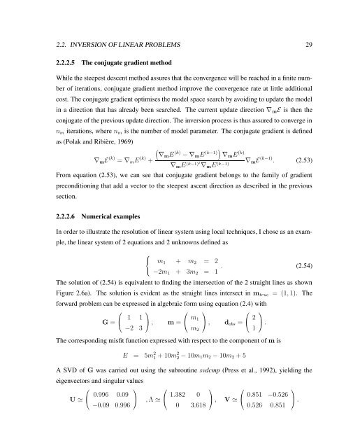
2.2.2.5 The conjugate gradient method
While the steepest descent method assures that the convergence will be reached in a finite number
of iterations, conjugate gradient method improve the convergence rate at little additional
cost. The conjugate gradient optimises the model space search by avoiding to update the model
in a direction that has already been searched. The current update direction ∇ m E is then the
conjugate of the previous update direction. The inversion process is thus assured to converge in
n m iterations, where n m is the number of model parameter. The conjugate gradient is defined
as (Polak and Ribière, 1969)
(
∇m E (k) − ∇
∇ m E (k) = ∇ m E (k) m E (k−1)) ∇ m E (k)
+
∇
∇ m E (k−1)t ∇ m E (k−1) m E (k−1) . (2.53)
From equation (2.53), we can see that conjugate gradient belongs to the family of gradient
preconditioning that add a vector to the steepest ascent direction as described in the previous
section.
2.2.2.6 Numerical examples
In order to illustrate the resolution of linear system using local techniques, I chose as an example,
the linear system of 2 equations and 2 unknowns defined as
⎧
⎨
⎩
m 1 + m 2 = 2
−2m 1 + 3m 2 = 1 . (2.54)
The solution of (2.54) is equivalent to finding the intersection of the 2 straight lines as shown
Figure 2.6a). The solution is evident as the straight lines intersect in m true
forward problem can be expressed in algebraic form using equation (2.4) with
⎛
G = ⎝ 1 1
⎞
⎛
⎠ , m = ⎝ m ⎞
⎛
1
⎠ , d obs = ⎝ 2 ⎞
⎠ .
−2 3
m 2 1
The corresponding misfit function expressed with respect to the component of m is
E = 5m 2 1 + 10m2 2 − 10m 1m 2 − 10m 2 + 5
= (1, 1). The
A SVD of G was carried out using the subroutine svdcmp (Press et al., 1992), yielding the
eigenvectors and singular values
⎛
⎞ ⎛
0.996 0.09
U ≃ ⎝ ⎠ , Λ ≃ ⎝ 1.382 0
⎞
⎠ ,
−0.09 0.996
0 3.618
⎛
⎞
0.851 −0.526
V ≃ ⎝ ⎠ .
0.526 0.851