Prediction Theory 1 Introduction 2 General Linear Mixed Model

Prediction Theory
1 Introduction
Best Linear Unbiased Prediction (BLUP) was developed for animal breeding by Dr. Charles
Roy Henderson around 1949. The methods were first applied to genetic evaluation of dairy sires
in the northeastern United States in 1970. BLUP is used in nearly all countries and all livestock
species for genetic evaluation of individual animals.
DEFINITION: Prediction is the estimation of the realized value of a random variable (from
data) that has been sampled from a population with a known variance-covariance structure.
2 General Linear Mixed Model
2.1 Equation of the Model
where
y = Xb + Zu + e
y is an N × 1 vector of observations,
b is a p × 1 vector of unknown constants,
u is a q × 1 vector of unknown effects of random variables,
e is an N × 1 vector of unknown residual effects,
X, Z are known matrices of order N × p and N × q respectively, that relate elements of b and
u to elements of y.
The elements of b are considered to be fixed effects while the elements of u are the random
effects from populations of random effects with known variance-covariance structures. Both b
and u may be partitioned into one or more factors depending on the situation.
2.2 Expectations and Covariance Structure
The expectations of the random variables are
E(u) = 0
1

E(e) = 0
E(y) = E(Xb + Zu + e)
= E(Xb) + E(Zu) + E(e)
= XE(b) + ZE(u) + E(e)
= Xb + Z0 + 0
= Xb
and the variance-covariance structure is typically represented as
( ) ( )
u G 0
V =
,
e 0 R
where G and R are known, positive definite matrices. Consequently,
V ar(y) = V ar(Xb + Zu + e)
Cov(y, u) = ZG
Cov(y, e) = R
= V ar(Zu + e)
= ZV ar(u)Z ′ + V ar(e) + ZCov(u, e) + Cov(e, u)Z ′
= ZGZ ′ + R, and
If u is partitioned into s factors as
u ′ =
(
u ′ 1 u ′ 2 · · · u ′ s
)
,
then
⎛
V ar(u) = V ar
⎜
⎝
Each G ij is assumed to be known.
u 1
u 2
.
u s
⎞ ⎛
⎟ = ⎜
⎠ ⎝
⎞
G 11 G 12 · · · G 1s
G ′ 12 G 22 · · · G 2s
.
. . .. ⎟ .
. ⎠
G ′ 1s G ′ 2s · · · G ss
3 Predictors
The problem is to predict the function
provided that K ′ b is an estimable function.
K ′ b + M ′ u,
2

3.1 Best Predictor
The best predictor, for any type of model, requires knowledge of the distribution of the random
variables as well as the moments of that distribution. Then, the best predictor is the conditional
mean of the predictor given the data vector, i.e.
E(K ′ b + M ′ u|y)
which is unbiased and has the smallest mean squared error of all predictors (Cochran 1951).
The computational form of the predictor depends on the distribution of y. The computational
form could be linear or nonlinear. The word best means that the predictor has the smallest
mean squared error of all predictors of K ′ b + M ′ u.
3.2 Best Linear Predictor
The best predictor may be linear OR nonlinear. Nonlinear predictors are often difficult to
manipulate or to derive a feasible solution. The predictor could be restricted to class of linear
functions of y. Then, the distributional form of y does not need to be known, and only the first
(means) and second (variances) moments of y must be known. If the first moment is Xb and
the second moment is V ar(y) = V, then the best linear predictor is
where
E(K ′ b + M ′ u) = K ′ b + C ′ V −1 (y − Xb)
C ′
= Cov(K ′ b + M ′ u, y).
When y has a multivariate normal distribution, then the best linear predictor (BLP) is the
same as the best predictor (BP). The BLP has the smallest mean squared error of all linear
predictors of K ′ b + M ′ u.
3.3 Best Linear Unbiased Predictor
In general, the first moment of y, namely Xb, is not known, but V, the second moment, is
commonly assumed to be known. Then predictors can be restricted further to those that are
linear and also unbiased. The best linear unbiased predictor is
where
and C and V are as before.
K ′ˆb + C ′ V −1 (y − Xˆb)
ˆb = (X ′ V −1 X) − X ′ V −1 y,
This predictor is the same as the BLP except that ˆb has replaced b in the formula. Note
that ˆb is the GLS estimate of b. Of all linear, unbiased predictors, BLUP has the smallest
mean squared error. However, if y is not normally distributed, then nonlinear predictors of
K ′ b + M ′ u could potentially exist that have smaller mean squared error than BLUP.
3

4 Derivation of BLUP
4.1 Predictand and Predictor
DEFINITION: The predictand is the function to be predicted, in this case
K ′ b + M ′ u.
DEFINITION: The predictor is the function to predict the predictand, a linear function of y,
i.e. L ′ y, for some L.
4.2 Requiring Unbiasedness
Equate the expectations of the predictor and the predictand to determine what needs to be true
in order for unbiasedness to hold. That is,
then to be unbiased for all possible vectors b,
E(L ′ y) = L ′ Xb
E(K ′ b + M ′ u) = K ′ b
L ′ X = K ′
or
L ′ X − K ′ = 0.
4.3 Variance of Prediction Error
The prediction error is the difference between the predictor and the predictand. The covariance
matrix of the prediction errors is
V ar(K ′ b + M ′ u − L ′ y) = V ar(M ′ u − L ′ y)
= M ′ V ar(u)M + L ′ V ar(y)L
−M ′ Cov(u, y)L − L ′ Cov(y, u)M
= M ′ GM + L ′ VL − M ′ GZ ′ L − L ′ ZGM
= V ar(P E)
4

4.4 Function to be Minimized
Because the predictor is required to be unbiased, then the mean squared error is equivalent
to the variance of prediction error. Combine the variance of prediction error with a LaGrange
Multiplier to force unbiasedness to obtain the matrix F, where
F = V ar(P E) + (L ′ X − K ′ )Φ.
Minimization of the diagonals of F is achieved by differentiating F with respect to the unknowns,
L and Φ, and equating the partial derivatives to null matrices.
∂F
∂L
= 2VL − 2ZGM + XΦ = 0
∂F
∂Φ = X′ L − K = 0
Let θ = .5Φ, then the first derivative can be written as
then solve for L as
VL = ZGM − Xθ
V −1 VL = L
= V −1 ZGM − V −1 Xθ.
Substituting the above for L into the second derivative, then we can solve for θ as
X ′ L − K = 0
X ′ (V −1 ZGM − V −1 Xθ) − K = 0
X ′ V −1 Xθ = X ′ V −1 ZGM − K
Substituting this solution for θ into the equation for L gives
θ = (X ′ V −1 X) − (X ′ V −1 ZGM − K)
L ′ = M ′ GZ ′ V −1 + K ′ (X ′ V −1 X) − X ′ V −1
−M ′ GZ ′ V −1 X(X ′ V −1 X) − X ′ V −1 .
Let
ˆb = (X ′ V −1 X) − X ′ V −1 y,
then the predictor becomes
L ′ y = K ′ˆb + M ′ GZ ′ V −1 (y − Xˆb)
which is the BLUP of K ′ b + M ′ u, and ˆb is a GLS solution for b. A special case for this predictor
would be to let K ′ = 0 and M ′ = I, then the predictand is K ′ b + M ′ u = u, and
L ′ y = û = GZ ′ V −1 (y − Xˆb).
( )
Hence the predictor of K ′ b + M ′ u is K ′ M ′ times the predictor of
(
ˆb′ û ′ ) ′
.
5
(
b ′
u ′ ) ′
which is

5 Variances of Predictors
Let
then
P = (X ′ V −1 X) −
ˆb = PX ′ V −1 y
û = GZ ′ V −1 (y − XPX ′ V −1 y)
= GZ ′ V −1 Wy
for W = (I − XPX ′ V −1 ). From the results on generalized inverses of X,
and therefore,
The variance of the predictor is,
The covariance between ˆb and û is
XPX ′ V −1 X = X,
WX = (I − XPX ′ V −1 )X
= X − XPX ′ V −1 X
= X − X = 0.
V ar(û) = GZ ′ V −1 W(V ar(y))W ′ V −1 ZG
= GZ ′ V −1 WVW ′ V −1 ZG
Therefore, the total variance of the predictor is
= GZ ′ V −1 ZG − GZ ′ V −1 XPX ′ V −1 ZG.
Cov(ˆb, û) = PX ′ V −1 V ar(y)W ′ V −1 ZG
= PX ′ W ′ V −1 ZG
= 0 because X ′ W = 0
V ar(K ′ˆb + M ′ û) = K ′ PK + M ′ GZ ′ V −1 ZGM
−M ′ GZ ′ V −1 XPX ′ V −1 ZGM.
6 Variance of Prediction Error
The main results are
V ar(ˆb − b) = V ar(ˆb) + V ar(b) − Cov(ˆb, b) − Cov(b, ˆb)
= V ar(ˆb)
= P.
V ar(û − u) = V ar(û) + V ar(u) − Cov(û, u) − Cov(u, û),
6

where
Cov(û, u) = GZ ′ V −1 WCov(y, u)
= GZ ′ V −1 WZG
= GZ ′ (V −1 − V −1 XPX ′ V −1 )ZG
= V ar(û)
so that
V ar(û − u) = V ar(û) + G − 2V ar(û)
= G − V ar(û).
Also,
Cov(ˆb, û − u) = Cov(ˆb, û) − Cov(ˆb, u)
= 0 − PX ′ V −1 ZG.
7 Mixed Model Equations
The covariance matrix of y is V which is of order N. N is usually too large to allow V to
be inverted. The BLUP predictor has the inverse of V in the formula, and therefore, would
not be practical when N is large. Henderson(1949) developed the mixed model equations for
computing BLUP of u and the GLS of b. However, Henderson did not publish a proof of these
properties until 1963 with the help of S. R. Searle, which was one year after Goldberger (1962).
Take the first and second partial derivatives of F,
( ) ( )
V X L
X ′ =
0 θ
Recall that V = V ar(y) = ZGZ ′ + R, and let
(
ZGM
K
)
which when re-arranged gives
S = G(Z ′ L − M)
M = Z ′ L − G −1 S,
then the previous equations can be re-written as
⎛
⎞ ⎛
R X Z
⎜
⎝ X ′ ⎟ ⎜
0 0 ⎠ ⎝
Z ′ 0 −G −1
L
θ
S
⎞
⎟
⎠ =
⎛
⎜
⎝
0
K
M
⎞
⎟
⎠ .
Take the first row of these equations and solve for L, then substitute the solution for L into
the other two equations.
L = −R −1 Xθ − R −1 ZS
7

and
( ) ( )
X
−
′ R −1 X X ′ R −1 Z
θ
Z ′ R −1 X Z ′ R −1 Z + G −1 S
=
(
K
M
Let a solution to these equations be obtained by computing a generalized inverse of
(
X ′ R −1 X X ′ R −1 Z
Z ′ R −1 X Z ′ R −1 Z + G −1 )
denoted as ( )
Cxx C xz
,
C zx C zz
then the solutions are
Therefore, the predictor is
L ′ y =
=
(
θ
S
(
(
)
= −
(
Cxx C xz
C zx C zz
) (
K
M
) ( ) (
K ′ M ′ C xx C xz X ′ R −1 y
C zx C zz Z ′ R −1 y
) ( ) ˆb
K ′ M ′ ,
û
)
.
)
)
.
where ˆb and û are solutions to
( ) (
X ′ R −1 X X ′ R −1 Z
ˆb
Z ′ R −1 X Z ′ R −1 Z + G −1 û
)
=
(
X ′ R −1 y
Z ′ R −1 y
)
.
The equations are known as Henderson’s Mixed Model Equations or MME. The equations are
of order equal to the number of elements in b and u, which is usually much less than the number
of elements in y, and therefore, are more practical to solve. Also, these equations require the
inverse of R rather than V, both of which are of the same order, but R is usually diagonal or
has a more simple structure than V. Also, the inverse of G is needed, which is of order equal
to the number of elements in u. The ability to compute the inverse of G depends on the model
and the definition of u.
The MME are a useful computing algorithm for obtaining BLUP of K ′ b + M ′ u. Please keep
in mind that BLUP is a statistical procedure such that if the conditions for BLUP are met,
then the predictor has the smallest mean squared error of all linear, unbiased predictors. The
conditions are that the model is the true model and the variance-covariance matrices of the
random variables are known without error.
In the strictest sense, all models approximate an unknown true model, and the variancecovariance
parameters are usually guessed, so that there is never a truly BLUP analysis of data,
except possibly in simulation studies.
8

8 Equivalence Proofs
The equivalence of the BLUP predictor to the solution from the MME was published by Henderson
in 1963. In 1961 Henderson was in New Zealand (on sabbatical leave) visiting Shayle
Searle learning matrix algebra and trying to derive the proofs in this section. Henderson needed
to prove that
V −1 = R −1 − R −1 ZTZ ′ R −1
where
and
T = (Z ′ R −1 Z + G −1 ) −1
V = ZGZ ′ + R.
Henderson says he took his coffee break one day and left the problem on Searle’s desk, and when
he returned from his coffee break the proof was on his desk.
VV −1 = (ZGZ ′ + R)(R −1 − R −1 ZTZ ′ R −1 )
= ZGZ ′ R −1 + I − ZGZ ′ R −1 ZTZ ′ R −1
−ZTZ ′ R −1
= I + (ZGT −1 − ZGZ ′ R −1 Z − Z)
TZ ′ R −1
= I + (ZG(Z ′ R −1 Z + G −1 )
−ZGZ ′ R −1 Z − Z)TZ ′ R −1
= I + (ZGZ ′ R −1 Z + Z
−ZGZ ′ R −1 Z − Z)TZ ′ R −1
= I + (0)TZ ′ R −1
= I.
Now take the equation for û from the MME
Z ′ R −1 Xˆb + (Z ′ R −1 Z + G −1 )û = Z ′ R −1 y
which can be re-arranged as
(Z ′ R −1 Z + G −1 )û = Z ′ R −1 (y − Xˆb)
or
The BLUP formula was
û = TZ ′ R −1 (y − Xˆb).
û = GZ ′ V −1 (y − Xˆb).
9

Then
GZ ′ V −1 = GZ ′ (R −1 − R −1 ZTZ ′ R −1 )
= (GZ ′ R −1 − GZ ′ R −1 ZTZ ′ R −1 )
= (GT −1 − GZ ′ R −1 Z)TZ ′ R −1
= (G(Z ′ R −1 Z + G −1 ) − GZ ′ R −1 Z)TZ ′ R −1
= TZ ′ R −1 .
Similarly, the MME solution for û and substituting it into the first equation in the MME
gives
X ′ R −1 Xˆb + X ′ R −1 Z(TZ ′ R −1 (y − Xˆb)) = X ′ R −1 y.
Combine the terms in ˆb and y to give
X ′ (R −1 − R −1 ZTZ ′ R −1 )Xˆb = X ′ (R −1 − R −1 ZTZ ′ R −1 )y,
which are the same as the GLS equations,
X ′ V −1 Xˆb = X ′ V −1 y.
Goldberger (1962) published these results before Henderson (1963), but Henderson knew of
these equivalences back in 1949 through numerical examples. After he discovered Goldberger’s
paper (sometime after his retirement) Henderson insisted on citing it along with his work. Most
people in animal breeding, however, refer to Henderson as the originator of this work and its
primary proponent.
9 Variances of Predictors and Prediction Errors From MME
The covariance matrices of the predictors and prediction errors can be expressed in terms of the
generalized inverse of the coefficient matrix of the MME, C. Recall that
( ) ( ) ( )
ˆb Cxx C
=
xz X ′ R −1
û C zx C zz Z ′ R −1 y,
or as
ˆb = C ′ by,
and
û = C ′ uy.
If the coefficient matrix of the MME is full rank (or a full rank subset) (to simplify the
presentation of results), then
( ) ( ) ( )
Cxx C xz X ′ R −1 X X ′ R −1 Z
I 0
C zx C zz Z ′ R −1 X Z ′ R −1 Z + G −1 =
,
0 I
10

which gives the result that
( ) (
Cxx C xz X ′ R −1 X X ′ R −1 Z
C zx C zz Z ′ R −1 X Z ′ R −1 Z
=
( )
I −Cxz G −1
0 I − C zz G −1 .
This last result is used over and over in deriving the remaining results.
Now,
V ar(ˆb) = V ar(C ′ by)
= C ′ bV ar(y)C b
= C ′ b(ZGZ ′ + R)C b
(
) ( )
X
= C xx C ′ R −1
xz
Z ′ R −1 (ZGZ ′ + R)C b
(
) ( )
X
= C xx C ′ R −1 Z
xz
Z ′ R −1 GZ ′ C
Z
b
(
+
C xx C xz
) ( X ′
Z ′ )
C b
)
= −C xz G −1 GZ ′ C b
(
) ( X
+ C xx C ′ R −1 X X ′ R −1 Z
xz
Z ′ R −1 X Z ′ R −1 Z
) ( )
Cxx
C zx
= C xz G −1 C zx
(
) ( )
+ I −C xz G −1 C xx
C zx
= C xz G −1 C zx + C xx − C xz G −1 C zx
= C xx .
The remaining results are derived in a similar manner. These give
V ar(û) = C u ′ V ar(y)C u
= G − C zz
Cov(ˆb, û) = 0
V ar(û − u) = V ar(û) + V ar(u) − Cov(û, u) − Cov(u, û)
= V ar(u) − V ar(û)
= G − (G − C zz )
= C zz
11

Cov(ˆb, û − u) = Cov(ˆb, u)
= C xz
In matrix form, the variance-covariance matrix of the predictors is
( ) ( )
ˆb Cxx 0
V ar =
,
û 0 G − C zz
and the variance-covariance matrix of prediction errors is
( ) ( )
ˆb
Cxx C
V ar
=
xz
.
û − u C zx C zz
As the number of observations in the analysis increases, two things can be noted from these
results:
1. V ar(û) increases in magnitude towards a maximum of G, and
2. V ar(û − u) decreases in magnitude towards a minimum of 0.
10 Hypothesis Testing
When G and R are assumed known, as in BLUP, then the solutions for ˆb from the MME
are BLUE and tests of hypotheses that use these solutions are best. Tests involving û are
unnecessary because when G and R have been assumed to be known, then the variation due
to the random factors has already been assumed to be different from zero. The general linear
hypothesis procedures are employed as in the fixed effects model. The null hypothesis is
( ) ( )
H ′ b
o 0 = c
u
or
H ′ ob = c,
where H ′ ob must be an estimable function of b and H ′ o must have full row rank.
estimable if
(
) ( )
H ′ X
o C xx C ′ R −1 X
xz
Z ′ R −1 = H ′
X
o.
The test statistic is
with r(H ′ o) degrees of freedom, and the test is
s = (H ′ oˆb − c) ′ (H ′ oC xx H o ) −1 (H ′ oˆb − c)
F = (s/r(H ′ o))/ˆσ 2 e,
H ′ ob is
where
ˆσ 2 e = (y ′ R −1 y − ˆb ′ X ′ R −1 y − û ′ Z ′ R −1 y)/(N − r(X)).
12

The degrees of freedom for F are r(H ′ o) and (N − r(X)). Note that
y ′ R −1 y − ˆb ′ X ′ R −1 y − û ′ Z ′ R −1 y = y ′ V −1 y − ˆb ′ X ′ V −1 y.
If G and R are not known, then there is no best test because BLUE of b is not possible.
Valid tests exist only under certain circumstances. If estimates of G and R are used to construct
the MME, then the solution for ˆb is not BLUE and the resulting tests are only approximate.
If the estimate of G is considered to be inappropriate, then a test of H ′ ob = c can be
constructed by treating u as a fixed factor, assuming that H ′ ob is estimable in the model with
u as fixed. That is,
( ) ( ) ˆb X
=
′ R −1 X X ′ R −1 − ( )
Z X ′ R −1 y
û Z ′ R −1 X Z ′ R −1 Z Z ′ R −1 ,
y
=
P zx P zz Z ′ R −1 y
(
Pxx P xz
) (
X ′ R −1 y
)
,
and
(
ˆσ e 2 = (y ′ R −1 y − ˆb ′ X ′ R −1 y − û ′ Z ′ R −1 y)/(N − r
X
Z
)
),
s = (H ′ oˆb − c) ′ (H ′ oP xx H o ) −1 (H ′ oˆb − c),
F = (s/r(H ′ o))/ˆσ 2 e.
11 Restrictions on Fixed Effects
There may be functions of b that are known and this knowledge should be incorporated into the
estimation process. For example, in beef cattle, male calves of a particular breed are known to
weigh 25 kg more than female calves of the same breed at 200 days of age. By incorporating a
difference of 25 kg between the sexes in an analysis then all other estimates of fixed and random
effects would be changed accordingly and also their variances.
Let B ′ b = d be the restriction to be placed on b, then the appropriate equations would be
⎛
X ′ R −1 X X ′ R −1 ⎞ ⎛ ⎞ ⎛
Z B ˆb X ′ R −1 ⎞
y
⎜
⎝ Z ′ R −1 X Z ′ R −1 Z + G −1 ⎟ ⎜ ⎟ ⎜
0 ⎠ ⎝ û ⎠ = ⎝ Z ′ R −1 ⎟
y ⎠ .
B ′ 0 0 φ
d
Because B ′ b = d is any general function, then there are three possible effects of this function
on the estimability of K ′ b in the model. The conditions on B ′ are that it
1. must have full row rank, and
2. must not have more than r(X) rows.
13

11.1 B ′ b is an estimable function
If B ′ b represents a set of estimable functions of b in the original model, then
1. the estimability of b is unchanged, and
2. the modified equations above do not have an inverse.
11.2 B ′ b is not an estimable function
If B ′ b represents a set of non-estimable functions of b with (p − r(X)) rows, where p is the
number of columns of X, then
1. b is estimable as if X was full column rank, and
2. the modified equations above have a unique inverse.
11.3 B ′ b is not an estimable function
If B ′ b represents a set of non-estimable functions of b with fewer than (p − r(X)) rows, and if
we let ( ) ( )
P11 P 12 X
=
′ V −1 −
X B
P 21 P 22 B ′ 0
then K ′ b is estimable if
(
K ′ 0
) ( ) (
P 11 P 12 X ′ V −1 X B
P 21 P 22 B ′ 0
=
(
K ′ 0
The modified MME do not have a unique inverse in this situation.
)
.
)
12 Restricted BLUP
BLUP is commonly applied to models to evaluate the genetic merit of livestock in order to make
decisions on culling and breeding of animals. In these cases, an objective of selection might be
to improve the performance of animals for one trait while leaving another trait unchanged. In
matrix notation, we might have two functions,
K ′ 1b + M ′ 1u and K ′ 2b + M ′ 2u,
14

epresenting the vectors of elements upon which selection decisions are to be made. One technique
of achieving the objective is to force the covariance between the predictor of one function
with the predictand of the other function to be zero. A zero covariance would result in no
correlated response in K ′ 2 b + M′ 2 u as a consequence of selecting on L′ 1y, provided y has a
multivariate normal distribution. The covariance matrix of concern is
Cov(L ′ 1y, K ′ 2b + M ′ 2u) = L ′ 1ZGM 2 .
Therefore, in deriving L ′ 1
we must add another LaGrange Multiplier to F to give
F = V ar(L ′ 1y − K ′ 1b − M ′ 1u) + (L ′ 1X − K ′ 1)Φ + L ′ 1ZGM 2 ϕ.
Minimize the diagonals of F with respect to L 1 , Φ, and ϕ, and equate the partial derivatives to
null matrices. The resulting modified MME would be
⎛
X ′ R −1 X X ′ R −1 Z X ′ R −1 ⎞ ⎛ ⎞
ZGM 2
ˆb
⎜
⎝ Z ′ R −1 X Z ′ R −1 Z + G −1 Z ′ R −1 ⎟ ⎜ ⎟
ZGM 2 ⎠ ⎝ û ⎠
M ′ 2 GZ′ R −1 X M ′ 2 GZ′ R −1 Z M ′ 2 GZ′ R −1 ZGM 2
ˆt
=
⎛
⎜
⎝
X ′ R −1 y
Z ′ R −1 y
M ′ 2 GZ′ R −1 y
⎞
⎟
⎠ .
Let a generalized inverse of the coefficient matrix be
⎛
⎞
C 11 C 12 C 13
⎜
⎟
⎝ C 21 C 22 C 23 ⎠ ,
C 31 C 32 C 33
then the following results may be derived:
V ar(ˆb) = C 11 ,
V ar(û − u) = C 22 ,
V ar(û) = G − C 22 ,
Cov(ˆb, û) = 0,
Cov(û, M ′ 2u) = 0,
Cov(ˆb, M ′ 2u) = 0,
Cov(ˆb, û − u) = C 12 ,
M ′ 2û = 0.
Another technique of obtaining the same result is to compute ˆb and û in the usual manner
from the MME, then derive the appropriate weights to apply, in K 1 and M 1 , such that
for a given M 2 .
Cov(K ′ 1ˆb + M ′ 1û, M ′ 2u) = 0,
15

13 Singular G
By definition, variance-covariance matrices should always be nonsingular. In particular, G and
R should be nonsingular because the MME utilize the inverse of these matrices to obtain BLUP.
The matrix V must always be nonsingular, but there may be cases when either G or R may be
singular.
Consider the case where G is singular, and therefore G does not have an inverse. The BLUP
of u is unaffected since the inverse of G is not needed, but in the MME there is a problem.
Harville (1976) and Henderson(1973) suggest pre-multiplying the last equation of the MME by
G to give ( )
)
X ′ R −1 X X ′ R −1 Z
GZ ′ R −1 X
GZ ′ R −1 Z + I
) ( ˆb
û
=
(
X ′ R −1 y
GZ ′ R −1 y
A disadvantage of these equations is that the coefficient matrix is no longer symmetric, and
solving the equations by Gauss-Seidel iteration may be slow to achieve convergence, if the
solutions converge at all. Also, the variance-covariance matrix of prediction errors has to be
obtained as follows:
V ar
( ˆb
û − u
)
=
(
X ′ R −1 X X ′ R −1 Z
GZ ′ R −1 X GZ ′ R −1 Z + I
) − (
I 0
0 G
.
)
.
The equations could be made symmetric as follows:
(
X ′ R −1 X X ′ R −1 ZG
) ( ) ˆb
GZ ′ R −1 X GZ ′ R −1 ZG + G ˆα
=
(
X ′ R −1 y
GZ ′ R −1 y
)
,
where
û = Gˆα,
and the variance-covariance matrix of prediction errors is calculated as
( ) ( ) ( )
ˆb
I 0 I 0
V ar
=
C
,
û − u 0 G 0 G
where C represents a generalized inverse of the coefficient matrix in the symmetric set of equations.
14 Singular R
When R is singular, the MME can not be used to compute BLUP. However, the calculation of
L ′ can still be used and the results given earlier on variances of predictors and prediction errors
still holds. The disadvantage is that the inverse of V is needed and may be too large to solve.
16

Another alternative might be to partition R and y into a full rank subset and analyze that part
ignoring the linearly dependent subset. However, the solutions for ˆb and û may be dependent
on the subsets that are chosen, unless X and Z may be partitioned in the same manner as R.
Singular R matrices do not occur frequently with continuously distributed observations, but
do occur with categorical data where the probabilities of observations belonging to each category
must sum to one.
15 When u and e are correlated
Nearly all applications of BLUP have been conducted assuming that Cov(u, e) = 0, but suppose
that Cov(u, e) = T so that
V ar(y) = ZGZ ′ + R + ZT ′ + TZ ′ .
A solution to this problem is to use an equivalent model where
y = Xb + Wu + ɛ
for
and
(
u
V ar
ɛ
W = Z + TG −1
)
=
(
G 0
0 B
)
where B = R − TG −1 T ′ , and consequently,
V ar(y) = WGW ′ + B
= (Z + TG −1 )G(Z ′ + G −1 T ′ ) + (R − TG −1 T ′ )
= ZGZ ′ + ZT ′ + TZ ′ + R
The appropriate MME for the equivalent model are
( ) (
X ′ B −1 X X ′ B −1 W
ˆb
W ′ B −1 X W ′ B −1 W + G −1 û
The inverse of B can be written as
)
=
(
X ′ B −1 y
W ′ B −1 y
)
.
but this form may not be readily computable.
B −1 = R −1 − R −1 T(G − T ′ R −1 T) −1 T ′ R −1 ,
The biggest difficulty with this type of problem is to define T = Cov(u, e), and then to
estimate the values that should go into T. A model with a non-zero variance- covariance matrix
between u and e can be re-parameterized into an equivalent model containing u and ɛ which
are uncorrelated.
17

16 G and R Unknown
For BLUP an assumption is that G and R are known without error. In practice this assumption
almost never holds. Usually the proportional relationships among parameters in these matrices
(i.e. such as heritabilities and genetic correlations) are known. In some cases, however, both G
and R may be unknown, then linear unbiased estimators of b and u may exist, but these may
not necessarily be best.
Unbiased estimators of b exist even if G and R are unknown. Let H be any nonsingular,
positive definite matrix, then
K ′ b o = K ′ (X ′ H −1 X) − X ′ H −1 y = K ′ CX ′ H −1 y
represents an unbiased estimator of K ′ b, if estimable, and
V ar(K ′ b o ) = K ′ CX ′ H −1 VH −1 XCK.
This estimator is best when H = V. Some possible matrices for H are I, diagonals of V,
diagonals of R, or R itself.
The u part of the model has been ignored in the above. Unbiased estimators of K ′ b can also
be obtained from
( ) ( ) ( )
X ′ H −1 X X ′ H −1 Z b
o X
Z ′ H −1 X Z ′ H −1 Z u o =
′ H −1 y
Z ′ H −1 y
provided that K ′ b is estimable in a model with u assumed to be fixed. Often the inclusion of u
as fixed changes the estimability of b.
If G and R are replaced by estimates obtained by one of the usual variance component
estimation methods, then use of those estimates in the MME yield unbiased estimators of b and
unbiased predictors of u, provided that y is normally distributed (Kackar and Harville, 1981).
Today, Bayesian methods are applied using Gibbs sampling to simultaneously estimate G and
R, and to estimate b and u.
17 Example 1
Below are data on progeny of three sires distributed in two contemporary groups. The first
number is the number of progeny, and the second number in parentheses is the sum of the
progeny observations.
Sire Contemporary Group
1 2
A 3(11) 6(19)
B 4(16) 3(18)
C 5(14)
18

17.1 Operational Models
Let
y ijk = µ + C i + S j + e ijk ,
where y ijk are the observations on the trait of interest of individual progeny, assumed to be one
record per progeny only, µ is an overall mean, C i is a random contemporary group effect, S j is
a random sire effect, and e ijk is a random residual error term associated with each observation.
E(y ijk ) = µ,
V ar(e ijk ) = σe
2
V ar(C i ) = σc 2 = σe/6.0
2
V ar(S j ) = σ 2 s = σ 2 e/11.5
The ratio of four times the sire variance to total phenotypic variance (i.e. (σ 2 c + σ 2 s + σ 2 e)), is
known as the heritability of the trait, and in this case is 0.2775. The ratio of the contemporary
group variance to the total phenotypic variance is 0.1329. The important ratios are
σ 2 e/σ 2 c = 6.0
σ 2 e/σ 2 s = 11.5
There are a total of 21 observations, but only five filled subclasses. The individual observations
are not available, only the totals for each subclass. Therefore, an equivalent model is the
“means” model.
ȳ ij = µ + C i + S j + ē ij ,
where ȳ ij is the mean of the progeny of the j th sire in the i th contemporary group, and ē ij is
the mean of the residuals for the (ij) th subclass.
The model assumes that
• Sires were mated randomly to dams within each contemporary group.
• Each dam had only one progeny.
• Sires were not related to each other.
• Progeny were all observed at the same age (or observations are perfectly adjusted for age
effects).
• The contemporary groups were independent from each other.
19

17.2 Mixed Model Equations
The process is to define y, X, and Z, and also G and R. After that, the calculations are
straightforward. The “means” model will be used for this example.
17.2.1 Observations
The observation vector for the “means” model is
⎛ ⎞
11/3
16/4
y =
14/5
.
⎜ ⎟
⎝ 19/6 ⎠
18/3
17.2.2 Xb and Zu
Xb =
⎛
⎜
⎝
1
1
1
1
1
⎞
⎟
⎠
µ.
The overall mean is the only column in X for this model.
There are two random factors and each one has its own design matrix.
where
so that, together,
Z c c =
⎛
⎜
⎝
1 0
1 0
1 0
0 1
0 1
Zu =
⎞
Zu =
(
Z c
Z s
) ( c
s
( )
C1
, Z
⎟ C s s =
⎠ 2
⎛
⎜
⎝
1 0 1 0 0
1 0 0 1 0
1 0 0 0 1
0 1 1 0 0
0 1 0 1 0
⎛
⎜
⎝
⎞ ⎛
⎟ ⎜
⎠ ⎝
)
,
1 0 0
0 1 0
0 0 1
1 0 0
0 1 0
C 1
C 2
S A
S B
S C
⎞
.
⎟
⎠
⎞
⎛
⎜
⎝
⎟
⎠
S A
S B
S C
⎞
⎟
⎠ ,
20

17.2.3 G and R
The covariance matrix of the means of residuals is R. The variance of a mean of random
variables is the variance of individual variables divided by the number of variables in the mean.
Let n ij equal the number of progeny in a sire by contemporary group subclass, then the variance
of the subclass mean is σe/n 2 ij . Thus,
R =
⎛
⎜
⎝
σ 2 e/3 0 0 0 0
0 σ 2 e/4 0 0 0
0 0 σ 2 e/5 0 0
0 0 0 σ 2 e/6 0
0 0 0 0 σ 2 e/3
⎞
.
⎟
⎠
The matrix G is similarly partitioned into two submatrices, one for contemporary groups
and one for sires.
( )
Gc 0
G =
,
0 G s
where
and
G c =
G s =
⎛
⎜
⎝
(
σ
2
c 0
0 σ 2 c
)
σ 2 s 0 0
0 σ 2 s 0
0 0 σ 2 s
⎞
= Iσ 2 c = I σ2 e
6.0 ,
⎟
⎠ = Iσ 2 s
= I σ2 e
11.5 .
and
The inverses of G and R are needed for the MME.
⎛
⎞
3 0 0 0 0
0 4 0 0 0
R −1 1
=
0 0 5 0 0
⎜
⎟ σ
⎝ 0 0 0 6 0 ⎠
2 ,
e
0 0 0 0 3
G −1 =
⎛
⎜
⎝
6 0 0 0 0
0 6 0 0 0
0 0 11.5 0 0
0 0 0 11.5 0
0 0 0 0 11.5
⎞
1
⎟ σ
⎠ e
2 .
Because both are expressed in terms of the inverse of σ 2 e, then that constant can be ignored.
The relative values between G and R are sufficient to get solutions to the MME.
21

17.2.4 MME and Inverse Coefficient Matrix
The left hand side of the MME (LHS) is
( ) (
X ′ R −1 X X ′ R −1 Z
ˆb
Z ′ R −1 X Z ′ R −1 Z + G −1 û
and the right hand side of the MME (RHS) is
(
X ′ R −1 y
Z ′ R −1 y
)
.
)
,
and
Numerically,
LHS =
⎛
⎜
⎝
21 12 9 9 7 5
12 18 0 3 4 5
9 0 15 6 3 0
9 3 6 20.5 0 0
7 4 3 0 18.5 0
5 5 0 0 0 16.5
RHS =
⎛
⎜
⎝
78
41
37
30
34
14
⎞
.
⎟
⎠
⎞ ⎛ ⎞
ˆµ
Ĉ 1
Ĉ 2
⎟
Ŝ ,
A
⎠ ⎜ ⎟
⎝ ŜB ⎠
ŜC
The inverse of LHS coefficient matrix is
⎛
⎞
.1621 −.0895 −.0772 −.0355 −.0295 −.0220
−.0895 .1161 .0506 .0075 .0006 −.0081
−.0772 .0506 .1161 −.0075 −.0006 .0081
C =
.
−.0355 .0075 −.0075 .0655 .0130 .0085
⎜
⎟
⎝ −.0295 .0006 −.0006 .0130 .0652 .0088 ⎠
−.0220 −.0081 .0081 .0085 .0088 .0697
C has some interesting properties.
• Add elements (1,2) and (1,3) = -.1667, which is the negative of the ratio of σ 2 c /σ 2 e.
• Add elements (1,4), (1,5), and (1,6) = -.08696, which is the negative of the ratio of σ 2 s/σ 2 e.
• Add elements (2,2) and (2,3), or (3,2) plus (3,3) = .1667, ratio of contemporary group
variance to residual variance.
• Add elements (4,4) plus (4,5) plus (4,6) = .08696, ratio of sire variance to residual variance.
Also, ( (5,4)+(5,5)+(5,6) = (6,4)+(6,5)+(6,6) ).
• The sum of ((4,2)+(5,2)+(6,2)) = ((4,3)+(5,3)+(6,3)) = 0.
22

17.2.5 Solutions and Variance of Prediction Error
Let SOL represent the vector of solutions to the MME, then
⎛ ⎞
ˆµ
( )
Ĉ 1
ˆb
SOL = C ∗ RHS = =
Ĉ 2
û
Ŝ A
⎜ ⎟
⎝ ŜB ⎠
ŜC
=
⎛
⎜
⎝
3.7448
−.2183
.2183
−.2126
.4327
−.2201
The two contemporary group solutions add to zero, and the three sire solutions add to zero.
The variances of prediction error are derived from the diagonals of C corresponding to the
random effect solutions multiplied times the residual variance. Hence, the variance of prediction
error for contemporary group 1 is .1161 σ 2 e. An estimate of the residual variance is needed. An
estimate of the residual variance is given by
ˆσ 2 e
= (SST − SSR)/(N − r(X)).
SST was not available from these data because individual observations were not available.
Suppose SST = 322, then
ˆσ 2 e = (322 − 296.4704)/(21 − 1) = 1.2765.
SSR is computed by multiply the solution vector times the RHS of the MME. That is,
SSR = 3.7448(78) − .2183(41) + .2183(37) − .2126(30) + .4327(34) − .2201(14) = 296.4704.
⎞
.
⎟
⎠
The variance of prediction error for contemporary group 1 is
V ar(P E) = .1161(1.2765) = .1482.
The standard error of prediction, or SEP, is the square root of the variance of prediction error,
giving .3850. Thus, the solution for contemporary group 1 is -.2183 plus or minus .3850.
Variances of prediction error are calculated in the same way for all solutions of random effects.
Effect Solution SEP
C 1 -.2183 .3850
C 2 .2183 .3850
S A -.2126 .2892
S B .4327 .2885
S C -.2201 .2983
Sire A has 9 progeny while sire B has 7 progeny, but sire B has a slightly smaller SEP. The
reason is due to the distribution of progeny of each sire in the two contemporary groups. Sire C,
of course, has the larger SEP because it has only 5 progeny and all of these are in contemporary
group 1. The differences in SEP in this small example are not large.
23

17.2.6 Repeatability or Reliability
Variances of prediction error are often expressed as a number going from 0 to 100 % , known as
repeatability or reliability (REL) (depending on the species). The general formula is
REL = (V ar(True Values) − V ar(P E))/(V ar(True Values),
times 100. Thus, for contemporary group 1, the reliability would be
For Sire A, the REL would be
REL = 100(.1667 − .1482)/(.1667) = 11.10.
REL = 100(.08696 − (.0655 ∗ 1.2765))/(.08696) = 3.85.
Thus, sires have smaller reliabilities than contemporary groups, but SEP for sires is smaller than
for contemporary groups. This is because contemporary groups have more progeny in them than
sires have, and because the variance of contemporary groups is larger than the variance of sire
transmitting abilities.
17.3 R Methods for MME
Given the matrices X, Z, G −1 , R −1 , and y, then an R-function can be written to set up the
MME, solve, and compute SSR. This function works for small examples, as given in these notes.
For large problems, other methods can be used to solve the equations by iterating on the data.
The function for small examples is given here.
24

MME = function(X,Z,GI,RI,y) {
XX = t(X) %*% RI %*% X
XZ = t(X) %*% RI %*% Z
ZZ = (t(Z) %*% RI %*% Z) + GI
Xy = t(X) %*% RI %*% y
Zy = t(Z) %*% RI %*% y
# Combine the pieces into LHS and RHS
piece1 = cbind(XX,XZ)
piece2 = cbind(t(XZ),ZZ)
LHS = rbind(piece1,piece2)
RHS = rbind(Xy,Zy)
# Invert LHS and solve
C = ginv(LHS)
SOL = C %*% RHS
SSR = t(SOL) %*% RHS
SOLNS = cbind(SOL,sqrt(diag(C)))
return(list(LHS=LHS,RHS=RHS,C=C,SSR=SSR,SOLNS=SOLNS))
}
To use the function,
Exampl = MME(X1,Z1,GI,RI,y)
str(Exampl)
# To view the results
Exampl$LHS
Exampl$RHS
Exampl$C
Exampl$SOLNS
Exampl$SSR
25

18 EXERCISES
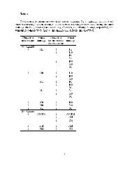
1. Below are data on progeny of 6 rams used in 5 sheep flocks (for some trait). The rams
were unrelated to each other and to any of the ewes to which they were mated. The first
number is the number of progeny in the herd, and the second (within parentheses) is the
sum of the observations.
Let the model equation be
Ram
Flocks
ID 1 2 3 4 5
1 6(638) 8(611) 6(546) 5(472) 0(0)
2 5(497) 5(405) 5(510) 0(0) 4(378)
3 15(1641) 6(598) 5(614) 6(639) 5(443)
4 6(871) 11(1355) 0(0) 3(412) 3(367)
5 2(235) 4(414) 8(874) 4(454) 6(830)
6 0(0) 0(0) 4(460) 12(1312) 5(558)
y ijk = µ + F i + R j + e ijk
where F i is a flock effect, R j is a ram effect, and e ijk is a residual effect. There are a total
of 149 observations and the total sum of squares was equal to 1,793,791. Assume that
σ 2 e = 7σ 2 f = 1.5σ2 r when doing the problems below.
(a) Set up the mixed model equations and solve. Calculate the SEPs and reliabilities of
the ram solutions.
(b) Repeat the above analysis, but assume that flocks are a fixed factor (i.e. do not add
any variance ratio to the diagonals of the flock equations). How do the evaluations,
SEP, and reliabilities change from the previous model
(c) Assume that rams are a fixed factor, and flocks are random.
similarly to the previous two models
Do the rams rank
2. When a model has one random factor and its covariance matrix is an identity matrix times
a scalar constant, then prove the the solutions for that factor from the MME will sum to
zero. Try to make the proof as general as possible.
26