Prediction Theory 1 Introduction 2 General Linear Mixed Model

16 G and R Unknown
For BLUP an assumption is that G and R are known without error. In practice this assumption
almost never holds. Usually the proportional relationships among parameters in these matrices
(i.e. such as heritabilities and genetic correlations) are known. In some cases, however, both G
and R may be unknown, then linear unbiased estimators of b and u may exist, but these may
not necessarily be best.
Unbiased estimators of b exist even if G and R are unknown. Let H be any nonsingular,
positive definite matrix, then
K ′ b o = K ′ (X ′ H −1 X) − X ′ H −1 y = K ′ CX ′ H −1 y
represents an unbiased estimator of K ′ b, if estimable, and
V ar(K ′ b o ) = K ′ CX ′ H −1 VH −1 XCK.
This estimator is best when H = V. Some possible matrices for H are I, diagonals of V,
diagonals of R, or R itself.
The u part of the model has been ignored in the above. Unbiased estimators of K ′ b can also
be obtained from
( ) ( ) ( )
X ′ H −1 X X ′ H −1 Z b
o X
Z ′ H −1 X Z ′ H −1 Z u o =
′ H −1 y
Z ′ H −1 y
provided that K ′ b is estimable in a model with u assumed to be fixed. Often the inclusion of u
as fixed changes the estimability of b.
If G and R are replaced by estimates obtained by one of the usual variance component
estimation methods, then use of those estimates in the MME yield unbiased estimators of b and
unbiased predictors of u, provided that y is normally distributed (Kackar and Harville, 1981).
Today, Bayesian methods are applied using Gibbs sampling to simultaneously estimate G and
R, and to estimate b and u.
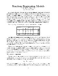
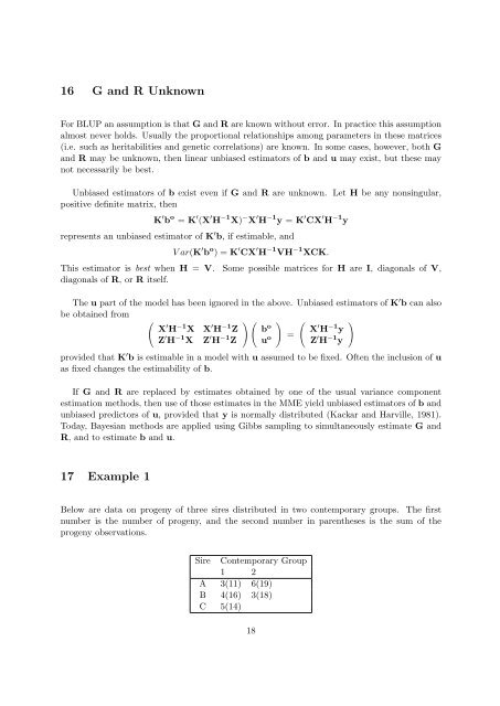
17 Example 1
Below are data on progeny of three sires distributed in two contemporary groups. The first
number is the number of progeny, and the second number in parentheses is the sum of the
progeny observations.
Sire Contemporary Group
1 2
A 3(11) 6(19)
B 4(16) 3(18)
C 5(14)
18