Prediction Theory 1 Introduction 2 General Linear Mixed Model

More documents

Recommendations

Info

17.2.4 MME and Inverse Coefficient Matrix The left hand side of the MME (LHS) is ( ) ( X ′ R −1 X X ′ R −1 Z ˆb Z ′ R −1 X Z ′ R −1 Z + G −1 û and the right hand side of the MME (RHS) is ( X ′ R −1 y Z ′ R −1 y ) . ) , and Numerically, LHS = ⎛ ⎜ ⎝ 21 12 9 9 7 5 12 18 0 3 4 5 9 0 15 6 3 0 9 3 6 20.5 0 0 7 4 3 0 18.5 0 5 5 0 0 0 16.5 RHS = ⎛ ⎜ ⎝ 78 41 37 30 34 14 ⎞ . ⎟ ⎠ ⎞ ⎛ ⎞ ˆµ Ĉ 1 Ĉ 2 ⎟ Ŝ , A ⎠ ⎜ ⎟ ⎝ ŜB ⎠ ŜC The inverse of LHS coefficient matrix is ⎛ ⎞ .1621 −.0895 −.0772 −.0355 −.0295 −.0220 −.0895 .1161 .0506 .0075 .0006 −.0081 −.0772 .0506 .1161 −.0075 −.0006 .0081 C = . −.0355 .0075 −.0075 .0655 .0130 .0085 ⎜ ⎟ ⎝ −.0295 .0006 −.0006 .0130 .0652 .0088 ⎠ −.0220 −.0081 .0081 .0085 .0088 .0697 C has some interesting properties. • Add elements (1,2) and (1,3) = -.1667, which is the negative of the ratio of σ 2 c /σ 2 e. • Add elements (1,4), (1,5), and (1,6) = -.08696, which is the negative of the ratio of σ 2 s/σ 2 e. • Add elements (2,2) and (2,3), or (3,2) plus (3,3) = .1667, ratio of contemporary group variance to residual variance. • Add elements (4,4) plus (4,5) plus (4,6) = .08696, ratio of sire variance to residual variance. Also, ( (5,4)+(5,5)+(5,6) = (6,4)+(6,5)+(6,6) ). • The sum of ((4,2)+(5,2)+(6,2)) = ((4,3)+(5,3)+(6,3)) = 0. 22
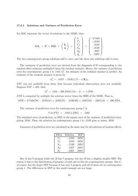
17.2.5 Solutions and Variance of <strong>Prediction</strong> Error Let SOL represent the vector of solutions to the MME, then ⎛ ⎞ ˆµ ( ) Ĉ 1 ˆb SOL = C ∗ RHS = = Ĉ 2 û Ŝ A ⎜ ⎟ ⎝ ŜB ⎠ ŜC = ⎛ ⎜ ⎝ 3.7448 −.2183 .2183 −.2126 .4327 −.2201 The two contemporary group solutions add to zero, and the three sire solutions add to zero. The variances of prediction error are derived from the diagonals of C corresponding to the random effect solutions multiplied times the residual variance. Hence, the variance of prediction error for contemporary group 1 is .1161 σ 2 e. An estimate of the residual variance is needed. An estimate of the residual variance is given by ˆσ 2 e = (SST − SSR)/(N − r(X)). SST was not available from these data because individual observations were not available. Suppose SST = 322, then ˆσ 2 e = (322 − 296.4704)/(21 − 1) = 1.2765. SSR is computed by multiply the solution vector times the RHS of the MME. That is, SSR = 3.7448(78) − .2183(41) + .2183(37) − .2126(30) + .4327(34) − .2201(14) = 296.4704. ⎞ . ⎟ ⎠ The variance of prediction error for contemporary group 1 is V ar(P E) = .1161(1.2765) = .1482. The standard error of prediction, or SEP, is the square root of the variance of prediction error, giving .3850. Thus, the solution for contemporary group 1 is -.2183 plus or minus .3850. Variances of prediction error are calculated in the same way for all solutions of random effects. Effect Solution SEP C 1 -.2183 .3850 C 2 .2183 .3850 S A -.2126 .2892 S B .4327 .2885 S C -.2201 .2983 Sire A has 9 progeny while sire B has 7 progeny, but sire B has a slightly smaller SEP. The reason is due to the distribution of progeny of each sire in the two contemporary groups. Sire C, of course, has the larger SEP because it has only 5 progeny and all of these are in contemporary group 1. The differences in SEP in this small example are not large. 23
Page 1 and 2: Prediction Theory 1 Introduction Be
Page 3 and 4: 3.1 Best Predictor The best predict
Page 5 and 6: 4.4 Function to be Minimized Becaus
Page 7 and 8: where Cov(û, u) = GZ ′ V −1 WC
Page 9 and 10: 8 Equivalence Proofs The equivalenc
Page 11 and 12: which gives the result that ( ) ( C
Page 13 and 14: The degrees of freedom for F are r(
Page 15 and 16: epresenting the vectors of elements
Page 17 and 18: Another alternative might be to par
Page 19 and 20: 17.1 Operational Models Let y ijk =
Page 21: 17.2.3 G and R The covariance matri
Page 25 and 26: MME = function(X,Z,GI,RI,y) { XX =

Prediction Theory 1 Introduction 2 General Linear Mixed Model

Create successful ePaper yourself

Delete template?

Save as template?