Prediction Theory 1 Introduction 2 General Linear Mixed Model
Prediction Theory 1 Introduction 2 General Linear Mixed Model
Prediction Theory 1 Introduction 2 General Linear Mixed Model

You also want an ePaper? Increase the reach of your titles
YUMPU automatically turns print PDFs into web optimized ePapers that Google loves.
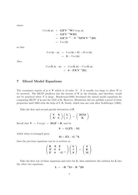
where<br />
Cov(û, u) = GZ ′ V −1 WCov(y, u)<br />
= GZ ′ V −1 WZG<br />
= GZ ′ (V −1 − V −1 XPX ′ V −1 )ZG<br />
= V ar(û)<br />
so that<br />
V ar(û − u) = V ar(û) + G − 2V ar(û)<br />
= G − V ar(û).<br />
Also,<br />
Cov(ˆb, û − u) = Cov(ˆb, û) − Cov(ˆb, u)<br />
= 0 − PX ′ V −1 ZG.<br />
7 <strong>Mixed</strong> <strong>Model</strong> Equations<br />
The covariance matrix of y is V which is of order N. N is usually too large to allow V to<br />
be inverted. The BLUP predictor has the inverse of V in the formula, and therefore, would<br />
not be practical when N is large. Henderson(1949) developed the mixed model equations for<br />
computing BLUP of u and the GLS of b. However, Henderson did not publish a proof of these<br />
properties until 1963 with the help of S. R. Searle, which was one year after Goldberger (1962).<br />
Take the first and second partial derivatives of F,<br />
( ) ( )<br />
V X L<br />
X ′ =<br />
0 θ<br />
Recall that V = V ar(y) = ZGZ ′ + R, and let<br />
(<br />
ZGM<br />
K<br />
)<br />
which when re-arranged gives<br />
S = G(Z ′ L − M)<br />
M = Z ′ L − G −1 S,<br />
then the previous equations can be re-written as<br />
⎛<br />
⎞ ⎛<br />
R X Z<br />
⎜<br />
⎝ X ′ ⎟ ⎜<br />
0 0 ⎠ ⎝<br />
Z ′ 0 −G −1<br />
L<br />
θ<br />
S<br />
⎞<br />
⎟<br />
⎠ =<br />
⎛<br />
⎜<br />
⎝<br />
0<br />
K<br />
M<br />
⎞<br />
⎟<br />
⎠ .<br />
Take the first row of these equations and solve for L, then substitute the solution for L into<br />
the other two equations.<br />
L = −R −1 Xθ − R −1 ZS<br />
7