Prediction Theory 1 Introduction 2 General Linear Mixed Model

More documents

Recommendations

Info

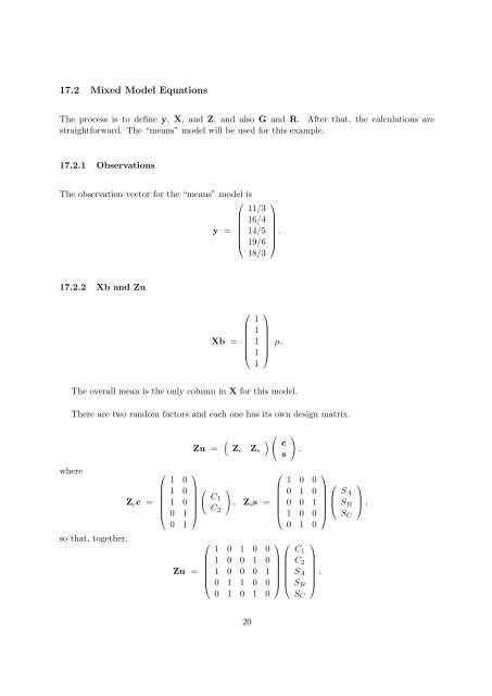
17.2 <strong>Mixed</strong> <strong>Model</strong> Equations The process is to define y, X, and Z, and also G and R. After that, the calculations are straightforward. The “means” model will be used for this example. 17.2.1 Observations The observation vector for the “means” model is ⎛ ⎞ 11/3 16/4 y = 14/5 . ⎜ ⎟ ⎝ 19/6 ⎠ 18/3 17.2.2 Xb and Zu Xb = ⎛ ⎜ ⎝ 1 1 1 1 1 ⎞ ⎟ ⎠ µ. The overall mean is the only column in X for this model. There are two random factors and each one has its own design matrix. where so that, together, Z c c = ⎛ ⎜ ⎝ 1 0 1 0 1 0 0 1 0 1 Zu = ⎞ Zu = ( Z c Z s ) ( c s ( ) C1 , Z ⎟ C s s = ⎠ 2 ⎛ ⎜ ⎝ 1 0 1 0 0 1 0 0 1 0 1 0 0 0 1 0 1 1 0 0 0 1 0 1 0 ⎛ ⎜ ⎝ ⎞ ⎛ ⎟ ⎜ ⎠ ⎝ ) , 1 0 0 0 1 0 0 0 1 1 0 0 0 1 0 C 1 C 2 S A S B S C ⎞ . ⎟ ⎠ ⎞ ⎛ ⎜ ⎝ ⎟ ⎠ S A S B S C ⎞ ⎟ ⎠ , 20
17.2.3 G and R The covariance matrix of the means of residuals is R. The variance of a mean of random variables is the variance of individual variables divided by the number of variables in the mean. Let n ij equal the number of progeny in a sire by contemporary group subclass, then the variance of the subclass mean is σe/n 2 ij . Thus, R = ⎛ ⎜ ⎝ σ 2 e/3 0 0 0 0 0 σ 2 e/4 0 0 0 0 0 σ 2 e/5 0 0 0 0 0 σ 2 e/6 0 0 0 0 0 σ 2 e/3 ⎞ . ⎟ ⎠ The matrix G is similarly partitioned into two submatrices, one for contemporary groups and one for sires. ( ) Gc 0 G = , 0 G s where and G c = G s = ⎛ ⎜ ⎝ ( σ 2 c 0 0 σ 2 c ) σ 2 s 0 0 0 σ 2 s 0 0 0 σ 2 s ⎞ = Iσ 2 c = I σ2 e 6.0 , ⎟ ⎠ = Iσ 2 s = I σ2 e 11.5 . and The inverses of G and R are needed for the MME. ⎛ ⎞ 3 0 0 0 0 0 4 0 0 0 R −1 1 = 0 0 5 0 0 ⎜ ⎟ σ ⎝ 0 0 0 6 0 ⎠ 2 , e 0 0 0 0 3 G −1 = ⎛ ⎜ ⎝ 6 0 0 0 0 0 6 0 0 0 0 0 11.5 0 0 0 0 0 11.5 0 0 0 0 0 11.5 ⎞ 1 ⎟ σ ⎠ e 2 . Because both are expressed in terms of the inverse of σ 2 e, then that constant can be ignored. The relative values between G and R are sufficient to get solutions to the MME. 21
Page 1 and 2: Prediction Theory 1 Introduction Be
Page 3 and 4: 3.1 Best Predictor The best predict
Page 5 and 6: 4.4 Function to be Minimized Becaus
Page 7 and 8: where Cov(û, u) = GZ ′ V −1 WC
Page 9 and 10: 8 Equivalence Proofs The equivalenc
Page 11 and 12: which gives the result that ( ) ( C
Page 13 and 14: The degrees of freedom for F are r(
Page 15 and 16: epresenting the vectors of elements
Page 17 and 18: Another alternative might be to par
Page 19: 17.1 Operational Models Let y ijk =
Page 23 and 24: 17.2.5 Solutions and Variance of Pr
Page 25 and 26: MME = function(X,Z,GI,RI,y) { XX =

Prediction Theory 1 Introduction 2 General Linear Mixed Model

Create successful ePaper yourself

Delete template?

Save as template?