Prediction Theory 1 Introduction 2 General Linear Mixed Model

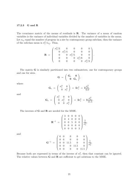
17.2.3 G and R
The covariance matrix of the means of residuals is R. The variance of a mean of random
variables is the variance of individual variables divided by the number of variables in the mean.
Let n ij equal the number of progeny in a sire by contemporary group subclass, then the variance
of the subclass mean is σe/n 2 ij . Thus,
R =
⎛
⎜
⎝
σ 2 e/3 0 0 0 0
0 σ 2 e/4 0 0 0
0 0 σ 2 e/5 0 0
0 0 0 σ 2 e/6 0
0 0 0 0 σ 2 e/3
⎞
.
⎟
⎠
The matrix G is similarly partitioned into two submatrices, one for contemporary groups
and one for sires.
( )
Gc 0
G =
,
0 G s
where
and
G c =
G s =
⎛
⎜
⎝
(
σ
2
c 0
0 σ 2 c
)
σ 2 s 0 0
0 σ 2 s 0
0 0 σ 2 s
⎞
= Iσ 2 c = I σ2 e
6.0 ,
⎟
⎠ = Iσ 2 s
= I σ2 e
11.5 .
and
The inverses of G and R are needed for the MME.
⎛
⎞
3 0 0 0 0
0 4 0 0 0
R −1 1
=
0 0 5 0 0
⎜
⎟ σ
⎝ 0 0 0 6 0 ⎠
2 ,
e
0 0 0 0 3
G −1 =
⎛
⎜
⎝
6 0 0 0 0
0 6 0 0 0
0 0 11.5 0 0
0 0 0 11.5 0
0 0 0 0 11.5
⎞
1
⎟ σ
⎠ e
2 .
Because both are expressed in terms of the inverse of σ 2 e, then that constant can be ignored.
The relative values between G and R are sufficient to get solutions to the MME.
21