Prediction Theory 1 Introduction 2 General Linear Mixed Model
Prediction Theory 1 Introduction 2 General Linear Mixed Model
Prediction Theory 1 Introduction 2 General Linear Mixed Model

Create successful ePaper yourself
Turn your PDF publications into a flip-book with our unique Google optimized e-Paper software.
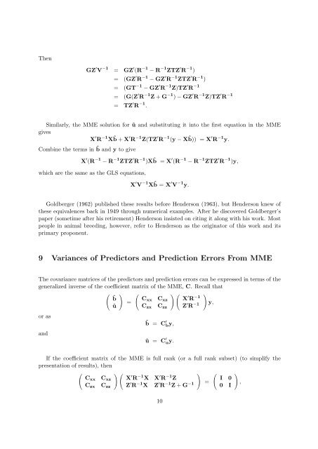
Then<br />
GZ ′ V −1 = GZ ′ (R −1 − R −1 ZTZ ′ R −1 )<br />
= (GZ ′ R −1 − GZ ′ R −1 ZTZ ′ R −1 )<br />
= (GT −1 − GZ ′ R −1 Z)TZ ′ R −1<br />
= (G(Z ′ R −1 Z + G −1 ) − GZ ′ R −1 Z)TZ ′ R −1<br />
= TZ ′ R −1 .<br />
Similarly, the MME solution for û and substituting it into the first equation in the MME<br />
gives<br />
X ′ R −1 Xˆb + X ′ R −1 Z(TZ ′ R −1 (y − Xˆb)) = X ′ R −1 y.<br />
Combine the terms in ˆb and y to give<br />
X ′ (R −1 − R −1 ZTZ ′ R −1 )Xˆb = X ′ (R −1 − R −1 ZTZ ′ R −1 )y,<br />
which are the same as the GLS equations,<br />
X ′ V −1 Xˆb = X ′ V −1 y.<br />
Goldberger (1962) published these results before Henderson (1963), but Henderson knew of<br />
these equivalences back in 1949 through numerical examples. After he discovered Goldberger’s<br />
paper (sometime after his retirement) Henderson insisted on citing it along with his work. Most<br />
people in animal breeding, however, refer to Henderson as the originator of this work and its<br />
primary proponent.<br />
9 Variances of Predictors and <strong>Prediction</strong> Errors From MME<br />
The covariance matrices of the predictors and prediction errors can be expressed in terms of the<br />
generalized inverse of the coefficient matrix of the MME, C. Recall that<br />
( ) ( ) ( )<br />
ˆb Cxx C<br />
=<br />
xz X ′ R −1<br />
û C zx C zz Z ′ R −1 y,<br />
or as<br />
ˆb = C ′ by,<br />
and<br />
û = C ′ uy.<br />
If the coefficient matrix of the MME is full rank (or a full rank subset) (to simplify the<br />
presentation of results), then<br />
( ) ( ) ( )<br />
Cxx C xz X ′ R −1 X X ′ R −1 Z<br />
I 0<br />
C zx C zz Z ′ R −1 X Z ′ R −1 Z + G −1 =<br />
,<br />
0 I<br />
10