Mathematica Tutorial: Dynamic Interactivity - Wolfram Research

Wolfram Mathematica ® Tutorial Collection 

DYNAMIC INTERACTIVITY

For use with Wolfram Mathematica ® 7.0 and later. 

For the latest updates and corrections to this manual: 

visit reference.wolfram.com 

For information on additional copies of this documentation: 

visit the Customer Service website at www.wolfram.com/services/customerservice 

or email Customer Service at info@wolfram.com 

Comments on this manual are welcomed at: 

comments@wolfram.com 

Content authored by: 

Theodore Gray and Lou D'Andria 

Printed in the United States of America. 

15 14 13 12 11 10 9 8 7 6 5 4 3 2 

©2008 Wolfram Research, Inc. 

All rights reserved. No part of this document may be reproduced or transmitted, in any form or by any means, 

electronic, mechanical, photocopying, recording or otherwise, without the prior written permission of the copyright 

holder. 

Wolfram Research is the holder of the copyright to the Wolfram Mathematica software system ("Software") described 

in this document, including without limitation such aspects of the system as its code, structure, sequence, 

organization, “look and feel,” programming language, and compilation of command names. Use of the Software unless 

pursuant to the terms of a license granted by Wolfram Research or as otherwise authorized by law is an infringement 

of the copyright. 

Wolfram Research, Inc. and Wolfram Media, Inc. ("Wolfram") make no representations, express, 

statutory, or implied, with respect to the Software (or any aspect thereof), including, without limitation, 

any implied warranties of merchantability, interoperability, or fitness for a particular purpose, all of 

which are expressly disclaimed. Wolfram does not warrant that the functions of the Software will meet 

your requirements or that the operation of the Software will be uninterrupted or error free. As such, 

Wolfram does not recommend the use of the software described in this document for applications in 

which errors or omissions could threaten life, injury or significant loss. 

Mathematica, MathLink, and MathSource are registered trademarks of Wolfram Research, Inc. J/Link, MathLM, 

.NET/Link, and webMathematica are trademarks of Wolfram Research, Inc. Windows is a registered trademark of 

Microsoft Corporation in the United States and other countries. Macintosh is a registered trademark of Apple 

Computer, Inc. All other trademarks used herein are the property of their respective owners. Mathematica is not 

associated with Mathematica Policy Research, Inc.

Contents 

Introduction to Dynamic . . . . . . . . . . . . . . . . . . . . . . . . . . . . . . . . . . . . . . . . . . . . . . . . . . . . . . . . . . 1 

Advanced Dynamic Functionality . . . . . . . . . . . . . . . . . . . . . . . . . . . . . . . . . . . . . . . . . . . . . . . . . 20 

Introduction to Manipulate . . . . . . . . . . . . . . . . . . . . . . . . . . . . . . . . . . . . . . . . . . . . . . . . . . . . . . . . 44 

Advanced Manipulate Functionality . . . . . . . . . . . . . . . . . . . . . . . . . . . . . . . . . . . . . . . . . . . . . . 104 

Generalized Input . . . . . . . . . . . . . . . . . . . . . . . . . . . . . . . . . . . . . . . . . . . . . . . . . . . . . . . . . . . . . . . . . . 126 

Views . . . . . . . . . . . . . . . . . . . . . . . . . . . . . . . . . . . . . . . . . . . . . . . . . . . . . . . . . . . . . . . . . . . . . . . . . . . . . . . 141

Introduction to Dynamic 

This tutorial describes the principles behind Dynamic, DynamicModule and related functions, 

and goes into detail about how they interact with each other and with the rest of Mathematica. 

These functions are the foundation of a higher-level function Manipulate that provides a simple 

yet powerful way of creating a great many interactive examples, programs, and demonstrations, 

all in a very convenient, though relatively rigid, structure. If that structure solves the 

problem at hand, you need look no further than Manipulate and you do not need to read this 

tutorial. However, do continue with this tutorial if you want to build a wider range of structures, 

including complex user interfaces. 

This is a hands-on tutorial. You are expected to evaluate all the input lines as you 

reach them and watch what happens. The accompanying text will not make sense 

without evaluating as you read. 

The Fundamental Principle of Dynamic 

Ordinary Mathematica sessions consist of a series of static inputs and outputs, which form a 

record of calculations done in the order in which they were entered. 

In[1]:= x = 5; 

Evaluate each of these four input cells one after the other. 

In[2]:= x 2 

Out[2]= 25 

In[1]:= x = 7; 

In[4]:= x 2 

Out[4]= 49 

The first output still shows the value from when x was 5, even though it is now 7. This is, of 

course, very useful, if you want to see a history of what you have been doing. However, you 

may often want a fundamentally different kind of output, one that is automatically updated to 

always reflect its current value. This new kind of output is provided by Dynamic. 

Evaluate the following cell; note that the result will be 49 because the current value of x is 7.

2 Dynamic Interactivity 

Evaluate the following cell; note that the result will be 49 because the current value of x is 7. 

In[5]:= 

DynamicAx 2 E 

In fact it is generally the case that when you first evaluate an input that contains variables 

wrapped in Dynamic, you will get the same result as you would have without Dynamic. But if 

you subsequently change the value of the variables, the displayed output will change 

retroactively. 

Evaluate the following cells one at a time, and note the change in the value displayed above. 

In[6]:= x = 9; 

In[7]:= x = 15; 

In[8]:= x = 10; 

The first two static outputs are still 25 and 49 respectively, but the single dynamic output now 

displays 100, the square of the last value of x. (This sentence will, of course, become incorrect 

as soon as the value of x is changed again.) 

There are no restrictions on the kinds of values that can go into a dynamic output. Just because 

x was initially a number does not mean it cannot become a formula or even a graphic in subsequent 

evaluations. This might seem like a simple feature, but it is the basis for a very powerful 

set of interactive capabilities. 

In[9]:= 

In[10]:= 

Each time the value of x is changed, the dynamic output above is updated automatically. (You 

might need to scroll back to see it.) 

1 

x = IntegrateB , yF; 

1 - y 3 

x = Plot@Sin@xD, 8x, 0, 2 Pi

Dynamic Interactivity 3 

Dynamic and Controls 

Dynamic is often used in connection with controls such as sliders and checkboxes. The full 

range of controls available in Mathematica is discussed in "Control Objects"; here sliders are 

used to illustrate how things work. The principles of using Dynamic with other controls is basically 

the same. 

A slider is created by evaluating the Slider function, in which the first argument is the position 

and the optional second argument specifies the range and step size, with the default range 

from 0 to 1 and the default step size 0. 

This is a slider in a centered position. 

In[11]:= 

Slider@0.5D 

Out[11]= 

Click on the thumb and move it around. The thumb moves, but nothing else happens since the 

slider is not connected to anything. 

In[12]:= 

This associates the position of the slider with the current value of the variable x. (This form is 

explained in more detail later.) 

Slider@Dynamic@xDD 

Out[13]= 

In[14]:= 

Out[14]= 0. 

This creates a new dynamic output of x since the last one has probably scrolled off your screen 

by now. 

Dynamic@xD 

Drag the last slider around. As the slider moves, the value of x changes and the dynamic output 

updates in real time. 

The slider also responds to changes in the value of x. 

To see this, evaluate this line. 

In[15]:= x = 0.8;


You should see the slider jump, and the dynamic output of x change, simultaneously. 

In[16]:= 

This creates another x slider. 


Out[16]= 

Notice that if you move either of the two sliders you now have, the other one moves in "lock 

sync." Both are connected, dynamically and bi-directionally, to the current value of x. 

Dynamic and Other Functions 

Dynamic and control constructs such as Slider are in many ways just like any other functions 

in Mathematica. They can occur anywhere in an output, in tables, and even inside typeset 

mathematical expressions. Wherever these functions occur, they carry with them the behavior 

of dynamically displaying or changing in real time the current value of the expression or variable 

they are linked to. Dynamic is a simple building block, but the rest of Mathematica turns it 

into a flexible tool for creating nimble, zippy, and often fun little interactive displays. 

This makes a table of x sliders, which are updated in sync. 

In[2]:= Table@Slider@Dynamic@xDD, 84 

In[3]:= 

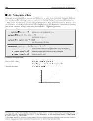
You can combine a slider with a display of its current value in a single output. 

8Slider@Dynamic@xDD, Dynamic@xD< 

Out[3]= : , 0.>


The great power of Dynamic lies in the fact that it can display any function of x just as easily. 

In[20]:= 

8Slider@Dynamic@xDD, Dynamic@Plot@Sin@10 y xD, 8y, 0, 2 Pi 

-0.5 

-1.0 

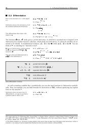
Using integer-valued sliders, you can create dynamically updated algebraic expressions. 

In[21]:= 

9Slider@Dynamic@x1D, 81, 10, 1 

In[22]:= 

You can use dynamic expressions with Panel, Row, Column, Grid, and other formatting 

constructs. 

Panel@Column@8Row@8Slider@Dynamic@xDD, Dynamic@xD


Localizing Variables in Dynamic Output 

In[23]:= 

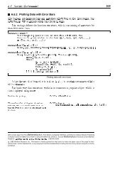
Here is another copy of a slider connected to a simple plot. 

8Slider@Dynamic@xDD, Dynamic@Plot@Sin@10 y xD, 8y, 0, 2 Pi 

-0.5 

-1.0 

In[24]:= 

This is a slider connected to another function. 

8Slider@Dynamic@xDD, Dynamic@Plot@Tan@10 y xD, 8y, 0, 2 Pi 

-0.5 

-1.0 

If you have both these outputs visible and drag either slider, you will notice that they are communicating 

with each other. Move the slider in one example, and the other example moves too. 

This is because you are using the global variable x in both examples. Although this can be very 

useful in some situations, most of the time you would probably be happier if these two sliders 

could be moved independently. The solution is a function called DynamicModule. 

DynamicModule@8x,y,…


DynamicModule has arguments identical to Module and is similarly used to localize and initialize 

variables, but there are important differences in how they operate. 

Here are the same two examples with "private" values of x. 

In[25]:= DynamicModule@8x = .5


Multiple DynamicModules can be placed in a single output, and they maintain separate values 

of the variables associated with their respective areas in the output. 

In[27]:= 8DynamicModule@8x = .5

in a new Mathematica session, the values of all the local variables will still be preserved and the 

sliders inside the DynamicModule will be in the same positions. This will not be the case with 


sliders linked to global variables (like the earliest examples in this tutorial), nor with sliders 

linked to variables localized with Module instead of DynamicModule. Such variables store their 

values in the current Mathematica kernel session, and they are lost as soon as you quit Mathematica. 

In addition to localizing variables to particular regions of output, DynamicModule provides 

options to automatically initialize function definitions when an expression containing a 

DynamicModule is opened, and to clean up values when the expression is closed or deleted. 

More details are found in DynamicModule. 

The Second Argument of Dynamic 

Dynamic connections are by default bi-directional. Sliders connected to a variable move 

together because they both reflect and control the value of the same variable. When you drag a 

slider thumb, the system constructs and evaluates expressions of the form expr = new, where 

expr is the expression given in the first argument to Dynamic and new is the proposed new value 

determined by where you have dragged the slider thumb. If the assignment can be done, the 

new value is accepted. If the assignment fails, the slider will not move. 

In[1]:= 

These two sliders move in opposite directions when you move the first one. However, trying to 

move the second slider gives an error because you cannot assign a new value to the expression 

1 - x. 

DynamicModule@8x = 0


In[30]:= 

This specifies how the value of x is to be updated and makes the second slider interactive. You 

can move either slider and the other slider responds by moving in the opposite direction. 



You can only move the thumb of this Slider2D along a circle. 

In[34]:= DynamicModule@8pt = 81, 0


In[37]:= 

But this does not. 

DynamicModule@8x


What is needed is a static slider, which contains within it a dynamic reference to the value of 

the variable. In the case of controls, there is a simple rule for where to put the Dynamic. The 

first argument of any control function, such as Slider, Checkbox, or PopupMenu, will almost 

always be Dynamic@varD. 

Beyond these cases where Dynamic will not work in a particular position, there is often a great 

deal of flexibility about where to place Dynamic. It is often used as the outermost function in an 

input expression, but this is by no means necessary, and in more sophisticated applications, 

Dynamic is usually used deeper in the expression and can even be nested. 

This displays a table of ten copies of the value of x. 

In[40]:= Dynamic@Table@x, 8i, 10


In[9]:= 

This is a tab view with two groups of dynamic expressions, both showing the dynamic values of 

x (a simple number) and y (a 3D plot). 

TabView@88Dynamic@xD, Dynamic@yD


In[10]:= h = 12; 

Dynamic can be wrapped around a whole Style expression. 

In[11]:= 

8Slider@Dynamic@hD, 86, 100 

Or Dynamic can be only in the FontSize option value. 

In[59]:= 

8Slider@Dynamic@hD, 86, 100 

There are two potential advantages to putting the Dynamic in the option value. First, suppose 

the dynamically regenerated expression is very large, for example if the block of text is the 

entire document, it is inefficient to retransmit it from the kernel to the front end every time the 

font size is changed, as is necessary if Dynamic encloses the whole expression. 

Second, the output of a Dynamic expression is not editable (since it is liable to be regenerated 

at any moment), which makes the output of the first example non-editable. But the text in the 

second example can be edited freely since it is ordinary static output: only the option value is 

dynamic. 

Dynamic option values can be also set in the Option Inspector. They are allowed at the cell, 

notebook, or global level, and in stylesheets. (Note, however, that if you set a dynamic option 

value in a position where the value will be inherited by many cells, for example in a stylesheet, 

there can be a significant impact on performance.) 

In[51]:= x = 0; 

You can set dynamic option values through SetOptions, as well. 

In[51]:= 

SetOptions@EvaluationNotebook@D, Background Ø Dynamic@Hue@xDDD 

In[52]:= 

Having linked the background color of the notebook to the global variable x, it can now be 

controlled by a slider or by a program. 


Out[52]= 

Of course, it is good to be able to return to normal. 

In[53]:= 

SetOptions@EvaluationNotebook@D, Background Ø InheritedD 

Dynamic and Infinite Loops


Dynamic and Infinite Loops 

If you are not careful, you can easily throw Dynamic into an infinite loop. 

In[54]:= 

This counts upwards as fast as possible for as long as it remains on screen. 



For example, suppose you have a list of numbers you wish to be able to modify by creating one 

slider to control each value. 

This creates the list and a dynamic display of its current value. 

In[1]:= data = 8.1, .5, .3, .9, .2

in a very surprising, though not technically incorrect, way with controls and other synchronous 


Slow Evaluations inside Dynamic 

Dynamic wrapped around an expression that will take forever, or even more than just a few 

seconds, to finish evaluating is a bad thing. 

In[61]:= 

If you evaluate this example, you will have to wait about 5 seconds before seeing the output 

$Aborted. 

Dynamic@While@TrueDD 

During the wait for the Dynamic output to evaluate, the front end is frozen, and no typing or 

other action is possible. Because updating of ordinary dynamic output locks up the front end, it 

is important to restrict the expressions you put inside Dynamic to things that will evaluate 

relatively quickly (preferably, within a second or so). Fortunately computers, and Mathematica, 

are fast, so a wide range of functions, including complex 2D and 3D plots, can easily be evaluated 

in a fraction of a second. 

To avoid locking up the front end for good, dynamic evaluations are internally wrapped in 

TimeConstrained, with a timeout value of, by default, 5 seconds. (This can be changed with 

the DynamicEvaluationTimeout option.) In certain extreme cases, TimeConstrained can fail to 

abort the calculation, in which case the front end will, a few seconds later, put up a dialog box 

allowing you to terminate dynamic updating until the offending output has been deleted. 

Fortunately there is an alternative if you need to have something slow in a Dynamic. The option 

SynchronousUpdating Ø False allows the dynamic to be evaluated in a way that does not lock 

up the front end. During evaluation of such an asynchronous Dynamic the front end continues 

operating as usual, but the main Shift +Return evaluation queue is occupied evaluating the 

Dynamic, so further Shift +Return evaluations will wait until the Dynamic finishes. (Normal 

synchronous Dynamic evaluations do not interfere with Shift +Return evaluations.) 

In[62]:= 

Evaluate this example, and you will see a gray placeholder rectangle for about 10 seconds, after 

which the result will be displayed. 

Dynamic@8DateList@D, Pause@10D; DateList@D


"Advanced Dynamic Functionality" gives more details about the differences between synchronous 

and asynchronous dynamic evaluations. In general, you should not plan to use asynchronous 

ones unless is it absolutely necessary. They do not update as quickly, and can interact 

in a very surprising, though not technically incorrect, way with controls and other synchronous 

evaluations. 

Further Reading 

The implementation details behind Dynamic and DynamicModule are worth understanding if you 

plan to use complex constructions, particularly those involving nested Dynamic expressions. 

This is discussed in "Advanced Dynamic Functionality".


Advanced Dynamic Functionality 

"Introduction to Manipulate" and "Introduction to Dynamic" provide most of the information you 

need to use Mathematica's interactive features accessible through the functions Manipulate, 

Dynamic, and DynamicModule. This tutorial gives further details on the workings of Dynamic 

and DynamicModule and describes advanced features and techniques for achieving maximum 

performance for complex interactive examples. 

Many examples in this tutorial display a single output value and use Pause to simulate slow 

calculations. In real life, you will instead be doing useful computations and displaying sophisticated 

graphics or large tables of values. 

Please note that this is a hands-on tutorial. You are expected to actually evaluate 

each of the input lines as you reach them in your reading, and watch what happens. 

The accompanying text will not make sense without evaluating as you read. 

Module versus DynamicModule 

Module and DynamicModule have similar syntax and in many respects behave similarly, at least 

at first glance. They are, however, fundamentally different in such areas as when their variables 

are localized, where the local values are stored, and in what universe the variables are unique. 

Module works by replacing all occurrences of its local variables with new, uniquely named 

variables, constructed so that they do not conflict with any variables in the current session of 

the Mathematica kernel. 

In[3]:= 

Out[3]= x$651 

You can see the names of these localized variables by allowing them to "escape" the context of 

the module without having been assigned a value. 

Module@8x


That is why sliders inside Module seem to work just as well as sliders inside DynamicModule. 

In[9]:= Table@Module@8x = .5 

In[10]:= Table@DynamicModule@8x = .5 

Both examples produce seemingly independent sliders that allow separate settings of separate 

copies of the variable x. The problem with sliders inside Module is that a different kernel session 

may coincidentally share the same localized variable names. So if this notebook is saved and 

then reopened sometime later, the sliders may "connect" to variables in some other Module 

that happen to have the same local variables at that time. 

This will not happen with the sliders inside DynamicModule because DynamicModule waits to 

localize the variables until the object is displayed in the front end and generates local names 

that are unique to the current session of the front end. Localization happens when 

DynamicModule is first created as output and then repeats anew each time the file that contains 

DynamicModule is opened, so there can never be a name conflict among examples generated in 

different sessions. 

Variables generated by Module are purely kernel session variables; when the kernel session 

ends, the values are irretrievably lost. DynamicModule, on the other hand, generates a structure 

in the output cell that is responsible for maintaining the values of the variables, allowing 

them to be saved in files. This is a somewhat subtle concept, best explained by way of two 

analogies. First, you can think of DynamicModule as a sort of persistent version of Module. 

Consider this command. 

In[5]:= 

ModuleA8x = 2, y, z


DynamicModule, on the other hand, creates an environment in which evaluations of expressions 

in Dynamic that appear within the body of the DynamicModule are like additional lines in the 

compound expression in the previous example. From one dynamic update to the next the 

values of all the variables are preserved, just as if the separate evaluations were separate lines 

in a compound expression, all within the local variable context created by DynamicModule. 

This preservation of variable values extends not just to subsequent dynamic evaluations within 

the same session, but to all future sessions. Because all the local variable values are stored and 

preserved in the notebook file, if the notebook is opened in an entirely new session of Mathemat - 

ica, the values will still be there, and dynamic updates will resume just where they left off. 

DynamicModule is like an indefinitely extendable Module. 

Another way to think about the difference between Module and DynamicModule is that while 

Module localizes its variables for a certain duration of time (while the body of the module is 

being evaluated), DynamicModule localizes its variables for a certain area of space in the output. 

As long as that space of the output remains in existence, the values of the variables defined for 

it will be preserved, allowing them to be used in subsequent evaluations of Dynamic expressions 

within the scope (area) of the DynamicModule. Saving the output into a file puts that bit 

of real estate into hibernation, waiting for the moment when the file is opened again. (In computer 

science terms, this is sometimes referred to as a freeze-dried or serialized object.) 

The ability of DynamicModule to preserve state across sessions is also a way of extending the 

notion of editing in a file. Normally when you edit text or expressions in a file, save the file, and 

reopen it, you expect it to open the way you left it. Editing means changing the contents of a 

file. 

Ordinary kernel variables do not have this property; if you make an assignment to x, then quit 

and restart Mathematica, x does not have that value anymore. There are several reasons for 

this, not least of which is the question of where the value of x should be saved. 

DynamicModule answers this question by defining a specific location (the output cell) where 

values of specific variables (the local variables) should be preserved. Arbitrary editing operations, 

like moving a slider, typing in an input field, or dragging a dynamic graphics object, 

change the values of the local variables. And since these values are automatically preserved 

when the file is saved, the sliders, and other objects, open exactly where they were left. Thus 

DynamicModule lets you make any quantity editable in the same way that text and expressions 

can be edited and saved in notebook files. 

Front End Ownership of DynamicModule Variable


Front End Ownership of DynamicModule Variable 

Values 

Ordinary variables in Mathematica are owned by the kernel. Their values reside in the kernel, 

and when you ask Mathematica to display the value in the front end, a transaction is initiated 

with the kernel to retrieve the value. The same is true of dynamic output that refers to the 

values of ordinary variables. 

In[6]:= x = 0; 

Consider this example. 

In[6]:= Table@Slider@Dynamic@xDD, 8500 

When one slider is moved, the other 499 move in sync with it. This requires 500 separate 

transactions with the kernel to retrieve the value of x. (The semantics of Mathematica are 

complex enough that there is no guarantee that evaluating x several times in a row will actually 

return the same value each time: it would not be possible for the front end to improve efficiency 

by somehow sharing a single value retrieved from the kernel with all the sliders.) 

Variables declared with DynamicModule, on the other hand, are owned by the front end. Their 

values reside in the front end, and when the front end needs a value, it can be retrieved locally 

with very little overhead. 

In[8]:= 

The following example thus runs noticeably faster. 


Whether it is better to use a normal kernel variable or a DynamicModule variable in a given 


situation depends on a number of factors. The most important is the fact that values of all 

DynamicModule variables are saved in the file when the notebook is saved. If you need a value 

preserved between sessions, it must be declared in a DynamicModule. On the other hand, a 

temporary variable holding a large table of numbers, for example, might be a poor choice for a 

DynamicModule variable as it could greatly increase the size of the file. It is quite reasonable to 

nest a Module inside a DynamicModule and vice versa, or to partition variables between the 

front end and kernel. 

In many situations the limiting factor in performance is the time needed to retrieve information 

from the kernel: by making variables local to the front end, speed can sometimes be increased 

dramatically. 

Automatic Updates of Dynamic Objects 

The specification for dynamic output is simple: Dynamic@exprD should always display the value 

you would get if you evaluated expr now. If a variable value, or some other state of the system, 

changes, the dynamic output should be updated immediately. Of course, for efficiency, not 

every dynamic output should be reevaluated every time any variable changes. It is critical that 

dependencies be tracked so that dynamic outputs are evaluated only when necessary. 

Consider these two expressions. 

In[9]:= Dynamic@a + b + cD 

Out[9]= a + b + c 

In[10]:= 

Dynamic@If@a, b, cDD 

Out[10]= If@a, b, cD 

The first expression might change its value any time the value of a, b, or c changes, or if any 

patterns associated with a, b, or c are changed. The second expression depends on a and b (but 

not c) while a is True and on a and c (but not b) while a is False. If a is neither True nor False, 

then it depends only on a (because the If statement returns unevaluated). 

Figuring out these dependencies a priori is impossible (there are theorems to this effect), so 

instead the system keeps track of which variables or other trackable entities are actually encoun - 

tered during the process of evaluating a given expression. Data is then associated with those 

variable(s) identifying which dynamic expressions need to be notified if the given variable 

receives a new value. 

An important design goal of the system is to allow monitoring of variable values by way of 

dynamic output referencing them, without imposing any more load than absolutely necessary 

on the system, especially if the value of the variable is being changed rapidly.


An important design goal of the system is to allow monitoring of variable values by way of 

dynamic output referencing them, without imposing any more load than absolutely necessary 

on the system, especially if the value of the variable is being changed rapidly. 

Consider this simple example. 

In[11]:= Dynamic@xD 

Out[11]= x 

In[13]:= Do@x, 8x, 1, 5 000 000


Dynamic outputs are only updated when they are visible on screen. This optimization allows 

you to have an open-ended number of dynamic outputs, all changing constantly, without incurring 

an open-ended amount of processor load. Outputs that are scrolled off-screen, above or 

below the current document position, will be left unexamined until the next time they are 

scrolled on-screen, at which point they are updated before being displayed. (Thus the fact that 

they stopped updating is not normally apparent, unless they have side effects, which is discouraged 

in general.) 

Dynamic output can depend on things other than variables, and in these cases tracking is also 

done carefully and selectively. 

This gives a rapidly updated display of the current mouse position in screen coordinates. 

In[14]:= Dynamic@MousePosition@DD 

Out[14]= 81058, 553< 

As long as the output is visible on screen, there will be a certain amount of CPU activity any 

time the mouse is moved, because this particular dynamic output is being redrawn immediately 

with every movement of the mouse. But if it is scrolled off-screen, the CPU usage will vanish. 

Refresh 

Normally, dynamic output is updated whenever the system detects any reason to believe it 

might need to be (see "Automatic Updates of Dynamic Objects" for details about what this 

means). Refresh can be used to modify this behavior by specifying explicitly what should or 

should not trigger updates. 

In[15]:= 

This updates when either slider is moved. 

DynamicModule@8x, y


In[16]:= 

This updates only when x changes, ignoring changes in y. 

DynamicModule@8x, y


This gives you a new number every second. 

In[17]:= 

Dynamic@Refresh@RandomReal@D, UpdateInterval Ø 1DD 

Out[17]= 0.722136 

In[18]:= 

Out[18]= $Failed 

This is not updated automatically. 

Dynamic@FileByteCount@ToFileName@ 

8$TopDirectory, "SystemFiles", "FrontEnd", "Palettes"


In[20]:= 

Out[20]= 9 

Consider this example. 

DynamicModule@8showclock = True


The example works, but now suppose you want to display the value of each number in the list 

next to its slider. 

You might at first try this. 

In[22]:= 

DynamicModule@8n = 5, data = Table@RandomReal@D, 820


Now you can drag any of the sliders and see dynamically updated values. This works because 

the outer Dynamic now depends only on the value of n, the number of sliders, not on the value 

of data. (Technically this is because Dynamic is HoldFirst: when it is evaluated, the expression 

in its first argument is never touched by evaluation, and therefore no dependencies are 

registered.) 

When building large, complex interfaces using multiple levels of nested Dynamic expressions, 

these are important issues to keep in mind. Mathematica works hard to do exactly the right 

thing even in the most complex cases. For example, the output of Manipulate consists of a 

highly complex set of interrelated and nested Dynamic expressions: if the dependency tracking 

system did not work correctly, Manipulate would not work right. 

Synchronous versus Asynchronous Dynamic 

Evaluations 

Mathematica consists of two separate processes, the front end and the kernel. These really are 

separate processes in the computer science sense of the word: two independent threads of 

execution with separate memory spaces that show up separately in a CPU task monitor. 

The front end and kernel communicate with each other through several MathLink connections, 

known as the main link, the preemptive link, and the service link. The main and preemptive 

links are pathways by which the front end can send evaluation requests to the kernel, and the 

kernel can respond with results. The service link works in reverse, with the kernel sending 

requests to the front end. 

The main link is used for Shift +Return evaluations. The front end maintains a queue of pending 

evaluation requests to send down this link. When you use Shift +Return on one or more input 

cells, they are all added to the queue, and then processed one by one. At any one time, the 

kernel is only aware of a single main link evaluation, the one it is currently working on (if any). 

In the meantime, the front end remains fully functional; you can type, open and save files, and 

so on. There is no arbitrary limit on how long a main link evaluation can reasonably take. People 

routinely do evaluations that take days to complete. 

The preemptive link works the same way as the main link in the sense that the front end can 

send an evaluation to it and get an answer, but it is administered quite differently on both 

Dynamic updates. 

There is no queue; instead, the front end sends one evaluation at a time and waits for the 

result before continuing with its other work. It is thus important to limit preemptive link evaluations 

to a couple of seconds at most. During any preemptive link evaluation, the front end is


ends. On the front end side, the preemptive link is used to handle normal Dynamic updates. 

There is no queue; instead, the front end sends one evaluation at a time and waits for the 

result before continuing with its other work. It is thus important to limit preemptive link evaluations 

to a couple of seconds at most. During any preemptive link evaluation, the front end is 

completely locked up, and no typing or other actions are possible. 

On the kernel side, evaluation requests coming from the preemptive link are given priority over 

evaluations from the main link, including the current running main link evaluation (if any). If an 

evaluation request comes from the preemptive link while the kernel is processing a main link 

evaluation, the main link evaluation is halted at a safe point (usually within microseconds). The 

preemptive link evaluation is then run to completion, after which the main link evaluation is 

restarted and allowed to continue as before. The net effect is similar to, though not the same 

as, a threading mechanism. Multiple fast preemptive link evaluations can be executed during a 

single long, slow main link evaluation, giving the impression that the kernel is working on more 

than one problem at a time. 

Preemptive link evaluations can change the values of variables, including those being used by a 

main link evaluation running at the same time. There is no paradox here, and the interleaving 

is done in a way that is entirely safe, though it can result in some fairly peculiar behavior until 

you understand what is going on. 

For example, evaluate this to get a slider. 

In[24]:= 


Out[24]= 

Then evaluate this command, and during the ten seconds it takes to finish, drag the slider 

around randomly. 

In[25]:= Table@Pause@1D; x, 810 False, you can tell the front end 

to use the main link queue, rather than the preemptive link. The front end then displays a gray 

box placeholder until it receives the response from the kernel.


Dynamic normally uses the preemptive link for its evaluations. Evaluation is synchronous, and 

the front end locks up until it is finished. This is unavoidable in some cases, but can be suboptimal 

in others. By setting the option SynchronousUpdating -> False, you can tell the front end 

to use the main link queue, rather than the preemptive link. The front end then displays a gray 

box placeholder until it receives the response from the kernel. 

In this case, the default (synchronous) update is appropriate because the front end needs to 

know the result of evaluating the Dynamic@xD for drawing with the correct font size. 

In[26]:= DynamicModule@8x = 12


Also, many controls need to be synchronous in order to be responsive to mouse actions. Making 

them asynchronous may cause potentially strange interactions with other controls. 

Here is a problematic example. 

In[30]:= n = 1; 

Column@8Slider@Dynamic@nD, 81, 10


ControlActive and SynchronousUpdatingÆAutomatic 

As a general rule, if you have a Dynamic that is meant to respond interactively to the movements 

of a slider or other continuous-action control, it should be able to evaluate in under a 

second, preferably well under. If the evaluation takes longer than that, you are not going to get 

satisfactory interactive performance, whether the Dynamic is updating synchronously or 

asynchronously. 

But what if you have an example that simply cannot finish evaluating fast enough, yet you want 

to be able to make it respond to a slider One option is to use asynchronous updating and 

simply accept that you will not get real-time interactive performance. If that is what you want 

to do, setting ContinuousAction -> False in the slider or other control is a good idea; that 

way you get only one update after the control is released, avoiding the starting up of potentially 

lengthy evaluations in the middle of a drag, before you have arrived at the value you want to 

stop at. 

The cell bracket becomes outlined, indicating evaluation activity, only after you release the 

slider. 

In[34]:= DynamicModule@8n = 1


The displayed text changes depending on whether or not the slider is being dragged. 

In[35]:= 

DynamicModule@8n = 1


This displays a 3D plot with a very small number of plot points while the control is being 

dragged and then refines the image with a large number of plot points when the control is 

released. 

In[37]:= DynamicModule@8n = 1


In addition, Manipulate uses SynchronousUpdating -> Automatic in Dynamic by default 

so the example becomes as simple as it can be. 

In[39]:= Manipulate@Plot3D@Sin@n x yD, 8x, 0, 3


Note first that Dynamic expressions with the default value of SynchronousUpdating -> True 

will never have a chance to use the value of their ImageSizeCache option, because they are 

always computed before being displayed, and, once computed, the actual image size will be 

used. 

On the other hand, Dynamic expressions with SynchronousUpdating Ø False will be displayed 

as a gray rectangle while they are being computed for the first time. In that case, the size of 

the rectangle is determined by the value of the ImageSizeCache option. This allows the surrounding 

contents of the notebook to be drawn in the right place, so that when the Dynamic 

finishes updating, there is no unnecessary flicker and shifting around of the contents of the 

notebook. (Users of HTML will recognize this as the analog of the width and height parameters 

of the img tag.) 

It is generally not necessary to specify the ImageSizeCache option explicitly, because the 

system will set it automatically as soon as the value of the Dynamic is computed successfully. 

(The computed result is measured, and the actual size copied into the ImageSizeCache option.) 

This automatically computed value is preserved if the Dynamic output is saved in a file. 

Consider the following input. 

In[40]:= Dynamic@Pause@3D; Style@"Hello", 100D, SynchronousUpdating Ø FalseD 

Out[40]=Hello 

When the input expression is evaluated, a small gray rectangle appears; because this Dynamic 

has never been evaluated, there is no cache of its proper image size, and a default small size is 

used. 

Three seconds later, the result arrives, and the dynamic output is displayed. At this point an 

actual size is known, and is copied to the ImageSizeCache option. You can see the value by 

clicking anywhere in the output cell and choosing Show Expression from the Cell menu. (This 

shows you the underlying expression representing the cell, exactly as it would appear in the 

notebook file if you were to save this cell.) Note the presence of an ImageSizeCache option. 

Now type a space in some innocuous place in the raw cell expression (to force a reparsing of 

the cell contents), and choose Show Expression again to reformat the cell. This time you will 

see a gray rectangle the size of the final output for three seconds, followed by the proper output. 

This is also what you would see if you opened a notebook containing previously saved, 

asynchronous dynamic output.


Now type a space in some innocuous place in the raw cell expression (to force a reparsing of 

the cell contents), and choose Show Expression again to reformat the cell. This time you will 

see a gray rectangle the size of the final output for three seconds, followed by the proper output. 

This is also what you would see if you opened a notebook containing previously saved, 

asynchronous dynamic output. 

The behavior of the setting SynchronousUpdating -> Automatic is similar, but subtly different. 

As we saw in the examples in "ControlActive and SynchronousUpdatingØAutomatic", with the 

Automatic setting, a synchronous preview-evaluation is done when the output is first placed, to 

provide a (hopefully) rapid display of the contents of the Dynamic expression before the slower, 

asynchronous value is computed. Because the first evaluation is synchronous, no gray rectangle 

is ever displayed. 

But this preview evaluation is done only if the ImageSizeCache option is not present. A Dynamic 

with SynchronousUpdating -> Automatic and an ImageSizeCache option specifying explicit 

dimensions will not do a synchronous preview evaluation, and will instead display a gray rectangle 

(of the correct size) pending the result of the first asynchronous evaluation. 

This may seem like baffling behavior at first, until you consider the practical effect of it. Generally 

speaking, Dynamic expressions will always have an ImageSizeCache option (created automatically 

by the front end) except for the very first time they appear, when they are originally 

placed as output from an evaluation. Any time they are opened from a file they will have a 

known, cached size. 

In Manipulate, which accounts for the vast majority of dynamic outputs, the default setting is 

SynchronousUpdating -> Automatic and the described behavior lets the output show up 

cleanly with a preview image in place when it is first generated. When a file containing dozens 

of Manipulate outputs is opened, you will get a useful behavior that is familiar from web 

browsers: the text displays immediately, and graphics (and other dynamic content) fill in later 

as fast as they are able. So you can scroll through a file rapidly, without any delay associated 

with precomputing potentially many preview images before the first page of the file can be 

displayed. 

If the initial evaluations when the Manipulate output was first placed were not synchronous, 

there would be flicker and resizing/shifting of the surroundings, because the size would not be 

known. But when the Manipulate output is opened from a file, the size is known, and the final 

output can be placed smoothly without flicker. 

One-Sided Updating of ControlActive


One-Sided Updating of ControlActive 

After evaluating in the kernel, ControlActive can trigger an update of the Dynamic containing 

it, but in a highly asymmetric fashion, only when it is going from the active to the inactive 

state. When making a transition in the other direction, from inactive to active, ControlActive 

does not trigger any update on its own. 

The reason for this somewhat unusual behavior is that ControlActive is a completely global 

concept. It returns the active state if any control anywhere in Mathematica is currently being 

dragged~even controls that have nothing to do with a particular Dynamic that happen to 

contain a reference to ControlActive. If ControlActive caused updates on its own, then as 

soon as you clicked any control, all Dynamic expressions containing references to 

ControlActive (e.g., a default dynamic Plot3D output) would immediately update, which 

would be entirely pointless. Instead, only those outputs that have some other reason for 

updating will pick up the current value of ControlActive. 

On the other hand, when the control is released, it is desirable to fix up any outputs that were 

drawn in control-active form, to give them their final polished appearance. Thus, when 

ControlActive is going into its inactive state, it needs to, on its own, issue updates to any 

Dynamic expression that may have been drawn in the active state. 

In[49]:= 

Dragging the slider does not change the Active/Inactive display because ControlActive does 

not trigger updates on its own. 

DynamicModule@8x


Now carefully release the mouse button without moving the mouse. Note that the display does 

revert to Inactive even though x has not changed. 

DynamicModule Wormholes 

The variables declared in a DynamicModule are localized to a particular rectangular area within 

one cell in a notebook. There are situations in which it is desirable to extend the scope of such 

a local variable to other cells or even other windows. For example, you might want to have a 

button in one cell that opens a dialog box that allows you to modify the value of a variable 

declared in the same scope as the button that opened the dialog. 

This can be done with one of the more surreal constructs in Mathematica, a DynamicModule 

wormhole. DynamicModule accepts the option DynamicModuleParent, whose value is a 

NotebookInterfaceObject that refers to another DynamicModule anywhere in the front end. 

For purposes of variable localization, the DynamicModule with this option will be treated as if it 

resided inside the one referred to, regardless of where the two actually are (even if they are in 

separate windows). 

The tricky part in setting up such a wormhole is getting the NotebookInterfaceObject necessary 

to refer to the parent DynamicModule. This reference can be created only after the 

DynamicModule has been created and placed as output, and it is valid only for the current 

session. 

To make the process easier, and in fact avoid all reference to explicit 

NotebookInterfaceObjects, DynamicModule also accepts the option InheritScope, which 

automatically generates the correct value of the DynamicModuleParent option to make the new 

DynamicModule function as if it were inside the scope of the DynamicModule from which it was 

created. This is confusing, so an example is in order. 

In[42]:= 

Evaluate this to create an output with a + button and a number. 



This - button is living in a wormhole created by the InheritScope option of the DynamicModule 

containing it. Clicking the button decrements the value of a local, private variable in the scope 

of a distant DynamicModule in another window. 

InheritScope can be used only when the code creating the second DynamicModule is executed 

from inside a button or other dynamic object located within the first DynamicModule. By using 

DynamicModuleParent explicitly, it is possible to link up arbitrary existing DynamicModules, but 

doing so is tricky, and beyond the scope of this document.


Introduction to Manipulate 

The single command Manipulate lets you create an astonishing range of interactive applications 

with just a few lines of input. Manipulate is designed to be used by anyone who is comfortable 

using basic commands such as Table and Plot: it does not require learning any complicated 

new concepts, nor any understanding of user interface programming ideas. 

The output you get from evaluating a Manipulate command is an interactive object containing 

one or more controls (sliders, etc.) that you can use to vary the value of one or more parameters. 

The output is very much like a small applet or widget: it is not just a static result, it is a 

running program you can interact with. 

This tutorial is designed for people who are familiar with the basics of using the Mathematica 

language, including how to use functions, the various kinds of brackets and braces, and how to 

make simple plots. Some of the examples will use more advanced functions, but it is not necessary 

to understand exactly how these work in order to get the point of the example. 

Despite the length of this tutorial, it is only half the story. "Advanced Manipulate Functionality" 

provides further information about some of the more sophisticated features of this rich 

command. 

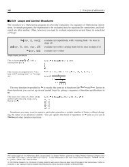
Manipulate Is as Easy as Table 

At its most basic, the syntax of Manipulate is identical to that of the humble function Table. 

Consider this Table command, which produces a list of numbers from one to twenty. 

Table@n, 8n, 1, 20


Manipulate@n, 8n, 1, 20


Note that the slider has an extra icon next to it which, when clicked, opens a small panel of 

additional controls. Here, the panel from the previous example is opened. 

n 

6.42 

1.0 

0.5 

1 2 3 4 5 6 

-0.5 

-1.0 

The panel allows you to see the numerical value of the variable, as well as set it in motion using 

the animation controls. 

If you want to see the value of the variable without having to open the subpanel, you can add 

the option Appearance -> "Labeled" to the variable specification. (Note the number displayed 

to the right of the plus sign, which is updated in real time as the slider is moved.) 

Manipulate@Plot@Sin@n xD, 8x, 0, 2 Pi


Just like Table, Manipulate allows you to give more than one variable range specification. 

Manipulate@Plot@Sin@n1 xD + Sin@n2 xD, 8x, 0, 2 Pi


You can open any or all of the subpanels to see numerical values, and you are free to animate 

many different variables at the same time if you like. 

One way to think of Manipulate is as a way to interactively explore a large parameter space. 

You can move around that space at will, exploring interesting directions as they appear. As you 

will see in later sections, Manipulate has many features designed to make such exploration 

easier and more rewarding. 

Symbolic Output and Step Sizes 

The previous examples are graphical, and indeed the most common application for Manipulate 

is producing interactive graphics. But Manipulate is capable of making any Mathematica function 

interactive, not just graphical ones. 

Often the first issue in examples involving symbolic, rather than graphical, output is that you 

want to deal with integers, rather than continuously variable real numbers. In Table the default 

step size is 1, so you naturally get integers, while in Manipulate the default is to allow continuous 

variation (which you could think of as a step size of zero). Compare these two examples, 

and note that Manipulate allows values in between those returned by Table. 

Table@n, 8n, 1, 20


Fortunately it is trivial to add an explicit step size of 1 to the Manipulate command, yielding 

exactly the same set of possible values in Manipulate as is returned by Table. 

Manipulate@n, 8n, 1, 20, 1


(In printed forms of this documentation, the slider is set fairly low to avoid wasting paper, but 

when moved all the way to the right, the output smoothly grows to cover many pages worth of 

vertical space.) 

As with Table, if you use rational numbers for the minimum and step, you will get perfect 

rational numbers in the variable, not approximate real numbers. Here is an example that uses 

the formatting function Row to create a simple example of adding fractions. 

Manipulate@Row@8n, "+", m, "=", n + m


The principle is that for each variable, you ask for a particular set of possible values, and 

Manipulate automatically chooses an appropriate type of control to make those values conveniently 

available. For a typical numerical Table-like iterator, a slider is the most convenient 

interface. 

You might, on the other hand, want to specify a discrete list of possible values (numeric or 

symbolic) rather than a range. This is done with an iterator of the form 

8variable, 8val1, val2, …


If you ask for a larger number of discrete values, Manipulate will switch to using a popup 

menu. 



These choices are of course somewhat arbitrary, but they are designed to be convenient, and 

you can always override the automatic choice of control type using a ControlType option 

inserted into the variable specification. (The full list of possible control types is given in the 

documentation for Manipulate.) 

For example, you can ask for a row of buttons even if the automatic behavior would have 

chosen a popup menu, using the option ControlType -> SetterBar. 



Sliders can be used to scan through discrete symbolic values, not just through numerical 

ranges (and this allows you to animate through them as well). The option 

ControlType -> Manipulator asks for the default control used by Manipulate, which is a 

slider plus an optional control panel with numerical value and animation controls (see the 

previous example). ControlType -> Slider asks for a plain slider. 



It is even possible to use two different controls to adjust the value of the same variable. Here 

both a popup menu and a slider are connected to the value of the filling variable. If the slider 

is used to select a value that does not appear in the popup menu, the popup will appear blank, 

but remains functional. When a value is chosen from the popup menu, the slider is moved to 

the corresponding position. Both controls can thus be used interchangeably to adjust the same 

value, and each one follows along when the other is being used. 



Initial Values and Labels 

Here is a fun example for making Lissajous figures. 

Manipulate@ParametricPlot@8a1 Sin@n1 Hx + p1LD, a2 Cos@n2 Hx + p2LD


Here is the same example with both amplitudes set to 1 initially, and the default frequency 

values set to give a pleasing initial figure. 



It is fun to watch how one shape turns into another, and in this connection it is good to know 

about an unusual feature of sliders in Mathematica. If you hold down the Option key 

(Macintosh) or Alt key (Windows), the action of the slider will be slowed down by a factor of 20 

relative to the movements of the mouse. In other words, when you drag the mouse left and 

right, the thumb will move only 1/20 th as much as it normally would. If you move outside the 

area of the slider, the value will start moving slowly in that direction as long as the mouse 

remains clicked. 

By holding down the Shift or Ctrl keys, or both, in addition to the Option/Alt key, you can slow 

the movement down by additional factors of 20 (one for each additional modifier key). With all 

three held down, it is possible to move the thumb by less that one part per million of its full 

range, which can be helpful in examples like this where beautiful patterns are hidden in very 

small ranges of parameter space. 

(The option PerformanceGoal -> "Quality" is used in this example to ensure that 

ParametricPlot draws smooth curves even when a slider is being moved: the need for this 

option is explained in more detail in "Advanced Manipulate Functionality".) 

By default Manipulate uses the names of the variables to label each control. But you may want 

to provide longer, more descriptive labels, which can be done by using variable specifications of 

the form 88var, init, label




When you have a small number of controls, it is usually most convenient to have them above 

the content area of the Manipulate panel. But because screens are typically wider than they 

are tall, if you have a large number of controls, you may find it better to put them on the left 

side, using the ControlPlacement option. 









The value of the variable will also be an 8x, y< pair. In this trivial example, just look at the 

value of the variable to get a feel for how the control works. 

Manipulate@pt, 8pt, 8-1, -1


To do something more interesting, you can recast the Lissajous figure from the previous section 

with three 2D sliders instead of six 1D sliders. You are controlling the same six parameters, but 

now you can do it two at a time. 

Manipulate@ 

ParametricPlot@8a@@1DD Sin@n@@1DD Hx + p@@1DDLD, a@@2DD Cos@n@@2DD Hx + p@@2DDLD


Graphics beyond Plotting 

So far high-level plotting functions have mostly been used, but it is equally interesting to use 

Mathematica's low level graphics language inside Manipulate. The following example, repeated 

from the previous section, is a trivial example of using the low-level graphics language. 

Manipulate@Graphics@8PointSize@0.1D, Point@ptD


Simple (or complicated) Mathematica programming can add arbitrary graphical elements to the 

output. For example, here we have lines to the center point instead of a dot, with a second 

linear slider determining the number of lines. 

Manipulate@ 

Graphics@8Line@Table@88Cos@tD, Sin@tD


Here is a fun little string-figure example also based on creating a table of lines. 

Manipulate@ 

Graphics@Line@Table@88Sin@n + iD, Cos@n + iD


Consider the previous example with lines going to a center point. While using a 2D slider is a 

fine way to control the center point, you might prefer to be able to simply click and drag the 

center point itself. This can be done by adding Locator to the control specification for the pt 

variable. In this case it is not necessary to specify a min and max range, because it can be taken 

automatically from the graphic. (It is, however, necessary to specify an initial value.) 

Manipulate@ 

Graphics@8Line@Table@88Cos@tD, Sin@tD


Manipulate@Graphics@Polygon@8pt1, pt2, pt3


Manipulate@Graphics@Polygon@ptsD, PlotRange Ø 1D, 

88pts, 880, 0


Manipulate@Graphics@Polygon@ptsD, PlotRange Ø 1D, 

88pts, 880, 0


Manipulate@ 

Graphics@8FaceForm@faceD, EdgeForm@8edge, Thickness@thicknessD


Manipulate@Module@8x


3D Graphics 

Manipulate can be used to explore 3D graphics just as easily as 2D, though performance 

issues become more of a concern. Consider this simple example. 

Manipulate@Plot3D@Sin@n x yD, 8x, 0, 3


The net result is that while you drag the slider, a fast, but somewhat crude, rendering of the 

plot is created in real time, and when you release the control, a smooth rendering shows up a 

moment later. (This happens because Plot3D, and most other plotting functions, refer to the 

function ControlActive in the default settings of the various options that control rendering 

quality and speed. See "Dealing with Slow Evaluations" in "Advanced Manipulate Functionality" 

for more about using ControlActive within Manipulate.) 

As in 2D, you can use the low-level graphics language just as easily as higher-level plotting 

commands. In this example you can see how Mathematica handles spheres that intersect with 

each other and with the bounding box. 

Manipulate@Graphics3D@8Sphere@80, 0, 0


This example shows how opacity (which is to say, transparency) can be used to see inside 

nested 3D structures. 

Manipulate@SphericalPlot3D@ q + f, 8q, 0, a p


All Types of Output Are Supported 

Manipulate is designed to work with the full range of possible types of output you can get with 

Mathematica, and it does not stop with graphical and algebraic output. Any kind of output 

supported by Mathematica can be used inside Manipulate. Here are some examples which may 

be less than obvious. 

Formatting constructs such as Grid, Column, Panel, etc. can be used to produce nicely formatted 

outputs. (See "Grids, Rows, and Columns" for more information about formatting 

constructs.) 

Manipulate@Grid@Table@8i, i^m


In this more complicated example the structure of a TabView is controlled by a Manipulate. 

Dynamic@paneD allows the current pane of the TabView to be selected either by using the slider 

created by Manipulate, or by clicking the TabView in the output area. The output is fully active. 

ManipulateBTabViewBTableBNestB 1 

&, base, iF, 8i, 1, n


Saving Definitions of Functions Used inside 

Manipulate 

Suppose you define a function, then use it in the first argument of a Manipulate. 

f@x_D := x^2 

Manipulate@f@yD, 8y, 0, 100 True, which causes it to automatically 

build into the Manipulate output a copy of all the definitions of functions referred to in the 

Manipulate input (and recursively any functions they refer to). These definitions are then 

reestablished in any new Mathematica sessions the Manipulate output is opened in, before 

contents of the Manipulate are evaluated for the first time. 

g@x_D := x^2 

Manipulate@g@yD, 8y, 0, 100


An alternative in such a case is to use the Initialization option to load a package of data 

from a file or other source, rather than building it into the Manipulate output. The 

Initialization option can be given any arbitrary block of Mathematica code to be evaluated 

before the contents of the Manipulate are first evaluated in any fresh session of Mathematica. 

The right-hand side of the Initialization option will be evaluated only once per session. 

For example, you can achieve the same result as earlier using the Initialization option 

instead of SaveDefinitions. 

Manipulate@h@yD, 8y, 0, 100


While Mathematica will work, or attempt to work, with any USB controller device (gamepad, 

joystick, simulated airplane throttle control~even data acquisition devices that use the USB 

controller interface standard), some definitely work better than others for controlling 

Manipulate outputs. Generally speaking, dual-joystick gamepads, such as commonly used with 

video games, provide a good set of controls, typically four analog axes and a large number of 

buttons. 

For the remainder of this section we will assume you are using a Logitech Dual Action gamepad. 

(This inexpensive controller is widely available and has better mechanical and electrical performance 

than many other units, even significantly more expensive ones.) If you are using a 

single joystick or another brand of gamepad there may be some differences in which controller 

parts map to which Manipulate parameters. 

With a gamepad plugged in, select the cell bracket of the cell containing the following output. 

Initially nothing will happen, because the gamepad's joysticks are in their neutral, undeflected 

position. But if you move them, you will see one or more of the parameters start to change. 

The rate at which the parameter changes is proportional to the degree of deflection of the 

joystick. 

Manipulate@Plot@a1 Sin@n1 xD + a2 Sin@n2 xD, 8x, 0, 2 Pi


By default, Manipulate connects the x axis of the left gamepad to the first parameter, the y 

axis of the left joystick to the second parameter, the x axis of the right joystick to the third 

parameter, and the y axis of the right gamepad to the fourth parameter. You can verify this by 

moving each joystick in a given direction and watching which parameter changes. (If you are 

using something other than a Logitech Dual Action gamepad you may see a different mapping: 

each manufacturer does things a bit differently, and while Mathematica has tables that attempt 

to normalize many commonly available controllers, new ones are always being introduced.) 

By default, the mapping is "velocity-based", which is to say that the rate at which the parameter 

changes is controlled by the position of the joystick. The joystick position is thus not directly 

connected to the value of the variable. 

You might instead want the value of the variable to be determined by the absolute position of 

the joystick, and there are two ways to achieve this. On many gamepads, including the recommended 

Logitech model, the joysticks are also buttons: if you press down on a joystick it clicks 

like a button, and when the joystick is controlling a Manipulate, this causes the corresponding 

parameter(s) to become directly linked to the position of the joystick. You can use this direct 

mode to rapidly jump to any position, then release the joystick to stop the parameter value 

there. 

If your gamepad does not have buttons in the joysticks, or you just want the linkage to always 

be direct, you can use the option ControllerMethod -> "Absolute".


Manipulate@Plot@a1 Sin@n1 xD + a2 Sin@n2 xD, 8x, 0, 2 Pi


Manipulate@Graphics@8Thickness@0.02D, 

Line@88-Cos@lD, Sin@lD


If you want a given Manipulate to always respond to the controller whether it is selected or 

not, you can add the option ControllerLinking -> All, but this feature should be used with 

caution. If you have multiple such outputs on screen, they will all attempt to move simultaneously, 

which is rarely helpful. The option is best used in situations where you are creating a 

fixed-format output window, rather than when creating examples meant to be used in a 

scrolling document such as this one. 

In examples like the previous one, which do not make much sense unless you have a gamepad 

available, it is often pointless to display the sliders associated with the parameters, or the rest 

of the framework of Manipulate. The function ControllerManipulate is basically identical to 

Manipulate in all its features and syntax, except that it does not display any frame or sliders. 

ControllerManipulate@Graphics@8Thickness@0.02D, 

Line@88-Cos@lD, Sin@lD


Manipulate will continue to be used in subsequent examples because it is helpful to be able to 

see the controls to understand how they are being affected by the gamepad, but many of these 

examples would look and work just as well with ControllerManipulate. 

If the Manipulate contains Slider2D variables, whose values are 8x, y< pairs of numbers, they 

will automatically be linked to both directions of available joysticks. This example responds in 

both directions to the left-hand joystick on a gamepad. 



Push buttons on the controller are by default linked up to any Boolean (True/False) parameters 

specified in the Manipulate. Which button is which can be a bit hard to guess on a given 

controller (a concept which is explained elsewhere), but on the Logitech model the group of 

four buttons on the right side are labeled 1 through 4, and are used by Manipulate in that 

order. In this example clicking the "1" button toggles the setting of b1, changing the color of 

the point. 

Manipulate@Graphics@8If@b1, Red, GreenD, PointSize@0.05D, Point@ptD


This toggling behavior (flipping the value of the parameter once each time the button is 

pressed) is the equivalent of velocity-based linking. If you use the 

ControllerMethod -> "Absolute" option (see previous examples) the parameter will be linked 

directly, which is to say its value will be False all the time except while the button is actually 

being held down. 

Manipulate@ 

Graphics@8If@b1, Red, GreenD, PointSize@0.05D, Point@ptD


The exact rules by which Manipulate connects controller axes to parameters are somewhat 

complex, but basically they try to allocate the available analog and Boolean controls to the 

parameters in the Manipulate so as to make maximum use of the available joysticks, buttons, 

knobs, and other widgets on the controller. (Often the quickest and easiest way to figure out 

what has been linked to what is simply to wiggle the various knobs and see what happens.) 

If you find that the default linking is not to your liking, it can be overridden by explicitly stating 

which controller axis should be connected to which parameter. The controller axes are named 

according to a logical system, but for most purposes it is enough to remember a few basic 

names: "X", "Y", "XY", "X1", "X2", "B1", "B2", etc. 

"X", or its synonym "X1", refers to the x axis of the primary, or the left-hand joystick on the 

gamepad. To specify that a parameter should be linked to this axis, use the following form. 

Manipulate@x, "X" Ø 8x, 0, 1


Axes can be combined into multidimensional parameters. For example, "XY" refers to both 

directions of the left or primary joystick, combined into a single 8x, y< value. Such a combined 

axis must be connected to a Slider2D style of parameter, as in this example. 



Three-axis variables are also supported as "XYZ". When using a three-axis joystick controller, 

the axes will correspond to the three degrees of freedom of the joystick. When using a dualjoystick 

gamepad, each joystick only has two degrees of freedom. In this case the "XYZ" axis is 

linked to the x and y directions of the left joystick plus the x direction of the right joystick. 

Whether this makes sense depends on the example: examples written specifically to take 

advantage of a three-degrees-of-freedom joystick may not work well with any other kind of 

controller. 

Manipulate@Graphics3D@8PointSize@0.05D, Point@ptD


Some controllers actually provide 6 analog degrees of freedom, which can be referred to as 

"XYZ" and "XYZ2". For example, if you have a 3Dconnexion SpaceNavigator control, the following 

example will let you explore its three spatial and three angular degrees of freedom. If you 

do not have one, the example will be unsatisfactory. 

Manipulate@ 

Graphics3D@8Thickness@0.01D, PointSize@0.04D, Point@pt1D, Line@8pt1, pt1 + pt2


A typical gamepad has two x-y controllers, named "XY" and "XY2". But what is less obvious is 

that there are also several more pseudo-analog axes available, generated by considering 

groups of four buttons as four directions: up, down, left, and right. For example, the "hat", a 

directional pad on the left side of a Logitech Dual Action gamepad, can be referenced as "XY3". 



These pseudo-analog axes act just like real analog ones, except that in velocity-linked mode 

they always progress at the same speed, and in absolute mode they are always pegged at the 

full-left, center, or full-right positions. 

When attempting to hook up specific axes it is often confusing trying to figure out which one is 

which on a given controller. The function ControllerInformation@D can be used to figure this 

out interactively. With your gamepad or joystick plugged in, evaluate this input (you have to 

evaluate it in your session of Mathematica with your controller plugged in to get current 

information). 

ControllerInformation@D 

Controller Device 1: Logitech Dual Action 

Controller Device 2: Apple IR 

Controller Device 3: Sudden Motion Sensor 

Depending on what type of computer you are using you may get several built-in controls. For 

example, Macintosh laptops typically contain a position sensor that reads out the orientation of 

the computer at all times. This information is available and can be used with Manipulate, but is 

not used by default (otherwise all Manipulate functions that run on such laptops would constantly 

move around as you tilted the computer, which some might consider a nuisance). 

Locate the controller you want to examine and click the disclosure triangle next to its name to 

open a panel of information, then open the Mathematica Controls subsection to see a list of 

all the available axis names.


ControllerInformation@D 

Controller Device 1: Logitech Dual Action 

Manufacturer Logitech H1133L 

Raw Product Name "Logitech Dual Action" 

Raw Product ID 49 686 

Device Type Mac OS X Human Interface Device 

Raw Controller Type Joystick 

Mathematica Controls 35 controls 

X 0.00392157 

Y 0.00392157 

Z 0.00392157 

X1 0.00392157 

Y1 0.00392157 

Z1 0.00392157 

X2 0.00392157 

Y2 -0.00392157 

X3 0. 

Y3 0. 

X4 0 

Y4 0 

X5 0 

Y5 0 

B1 False 

B2 False 

B3 False 

B4 False 

B5 False 

B6 False 

B7 False 

B8 False 

B9 False 

B10 False 

B11 False 

B12 False 

BLB False 

BRB False 

JB False 

JB1 False 

JB2 False 

Select Button False 

Start Button False 

TLB False 

TRB False 

Show Dynamic Values 

Raw Controls 

18 controls 

Controller Device 2: Apple IR 

Controller Device 3: Sudden Motion Sensor 

If Show Dynamic Values is checked, the values displayed in the panel will update in real time 

as you wiggle the controller or push its buttons, allowing you to easily determine which button 

corresponds to which named axis. (Do not forget the quotes around the axis names when using


If Show Dynamic Values is checked, the values displayed in the panel will update in real time 

as you wiggle the controller or push its buttons, allowing you to easily determine which button 

corresponds to which named axis. (Do not forget the quotes around the axis names when using 

them in Manipulate.) 

The option ControllerMethod can only be used at the level of the whole Manipulate to change 

the linking from velocity-based to absolute. If you want to make some axes absolute and some 

velocity-based, add "Absolute" to the name of any axes you want to have linked absolutely, as 

in this example, which has a velocity-based x direction and an absolute y direction. 

Manipulate@Graphics@8PointSize@0.05D, Point@8x, y


Autorun 

In many ways Manipulate is a big improvement over simple linear animations. Rather than 

running through a fixed sequence, Manipulate lets you move back and forth at will. But what if 

you do not want to have to move a slider by hand One option is to use the icon next to each 

slider to open a panel with animation controls. A Manipulate with one variable being animated 

is virtually equivalent to Animate. 

But if you have multiple variables and want to see the effect of changing all of them, it is inconvenient 

to use the individual animation controls. The Autorun feature of Manipulate solves 

this problem by providing a single animation control that runs all the variables through their 

ranges of values. 

Click the menu in the top right corner of a Manipulate output and select Autorun from the 

bottom of the menu. You will see an Autorun panel appear at the top of the Manipulate, 

containing animation controls and a button. By default the animation runs each individual 

variable through its range of values, leaving the others at their default values. As with any 

animation control, you can change the speed and direction, or click the slider to move through 

the animation manually. The Autorun animation slider acts as a sort of master control driving 

all the other controls in a defined order.






AutorunSequencing allows you to specify the duration reserved for the animation of a particular 

control. This setting reserves two seconds for the first control, two seconds for the third 

control, and ten seconds for the fourth control. The second control is skipped as before. 

Manipulate@8w, x, y, z


To get a single value out into a form you can use as a static input, use the Paste Snapshot 

command from the menu. The result will be inserted as a new cell below the Manipulate 

output. 

Manipulate@8x, y, z


Bookmarks are lists of locations in a given parameter space, and you can extract the raw data 

in that list by choosing the Paste Bookmarks item. Every element of the resulting list is of the 

form bookmarkName :> parameterValues. This list is syntactically appropriate for reinserting 

into Manipulate input as the setting for the Bookmarks option. (This allows you to, for example, 

modify the bookmarks by manual editing, or run a program on them, before restoring them 

as active bookmarks in a new Manipulate output.) 

The Animate Bookmarks menu command works much like the Autorun command described 

in the previous section, except that instead of animating each parameter through its range of 

values, it creates an animation that interpolates through the points specified by the bookmarks. 

The interpolation which occurs when animating bookmarks is done internally via the 

Interpolation command. Manipulate even accepts the InterpolationOrder option to adjust 

how the animation proceeds from one point to the next. The default value of Automatic performs 

quadratic interpolation if there are enough bookmarks, and linear interpolation otherwise. 

When a Manipulate output containing explicit bookmarks is exported to a video animation 

format using Export, the resulting video will be one cycle through the sequence generated by 

Animate Bookmarks. (If no bookmarks are present, the result is one cycle of Autorun.)


Advanced Manipulate Functionality 

This tutorial covers advanced features of the Manipulate command. It assumes that you have 

read "Introduction to Manipulate" and thus have a good idea what the command is for and how 

it works overall. 

This tutorial also, in places, assumes a familiarity with the lower-level dynamic mechanism 

covered in "Introduction to Dynamic" and "Advanced Dynamic Functionality". 

Please note that this is a hands-on tutorial. You are expected to actually evaluate 

each input line as you reach it in your reading, and watch what happens. The accompanying 

text will not make sense without evaluating as you read. 

Controlling Automatic Reevaluation 

Some Manipulate examples "spin," continually reevaluating their contents even when no 

sliders are being moved. Sometimes this is in fact exactly what you intend. For example, here 

is a droopy triangle, which always sags down in the middle. You can drag it back up using the 

slider, but as soon as you stop moving, it starts falling down again.


Manipulate@ 

y = Max@-1, y - 0.05D; Graphics@Polygon@88-1, 1


Manipulate@total = total + step; 8step, total


Manipulate@Module@8f


In[26]:= 

Manipulate@With@8value = Table@c@iD, 8i, 1, n


You might wonder why m is not automatically reset to the current maximum, when the maximum 

is set lower than its current value. The reason is that sometimes it is preferable to leave 

the value alone, and if you want to have it reset automatically, it is easy to do manually. For 

example, you can add an If statement to the code in the first argument. 

Manipulate@If@m > n, m = nD; 

Row@8"H", Column@8n, m


Dealing with Slow Evaluations 

Manipulate does not precompute all the possible output values you could reach by moving its 

sliders: that would be completely impractical for all but the most trivial cases. That means it 

has to calculate, format, and display the current value in real time as each slider is being 

dragged. Obviously no matter how fast your computer, there is a limit to how much computation 

can be done in a finite amount of time, and if the expression you use in the first argument 

to Manipulate takes more than about a second to evaluate, you will not have a very satisfactory 

experience using the Manipulate. 

Many very interesting and powerful computations can be done in under a second, and as computers 

get faster the range will only increase (people are not getting any faster, so the amount of 

time available before the example seems too sluggish should remain unchanged for quite a 

while). But some computations just cannot be done that fast, and some alternative is necessary 

if you want to use them within Manipulate. Fortunately there are several good ways of dealing 

with slow evaluations. 

For purposes of this section we are going to use Pause to simulate a slow evaluation. The main 

reason for this is that any actual computation would run at such widely differing speeds on 

different users' computers that it would be hard to illustrate the point with any one example. So 

where you see a Pause command, please imagine that something terribly complex and interesting 

is being done, resulting in a fantastically detailed and enlightening output. 

To get a feel for the problem, try dragging the following slider. While this example is not unacceptable, 

it is on the borderline of something not worth playing with. If the delay is increased to 

several seconds, it becomes quite pointless. (And beyond 5 seconds you will start seeing 

$Aborted instead of the number, because the system is protecting itself from unreasonably 

long evaluations, which block other activity in the front end in this situation.) 

Manipulate@Pause@1D; x, 8x, 0, 10


The simplest improvement is to add the option ContinuousAction -> False to the Manipulate. 

Manipulate@Pause@1D; x, 8x, 0, 10 False option, arbitrarily long 

evaluations can be used. (Though something that takes a minute is still probably better done as 

a normal Shift+Return evaluation than inside Manipulate.) 

A more sophisticated alternative is to use the ControlActive function to present an alternative, 

simpler and faster display while the slider is being dragged, and do the long computation 

only when it is released. 

ControlActive takes two arguments: the first is returned if the expression is evaluated while a 

control (e.g. a slider) is currently being dragged with the mouse, and the second if no control is 

currently active. (See the documentation for ControlActive for some fine print about exactly 

when which argument is returned.) 

In this example we use just x as the preview to be displayed while the slider is being dragged, 

and x with a box around it, plus a second of delay, as the final display to be presented when 

the slider is released. Note that we have removed the ContinuousAction -> False option from 

the example above.


Manipulate@ControlActive@x, Pause@1D; Framed@xDD, 8x, 0, 10


But even the higher number used after the slider is released is not enough to produce a satisfactory 

plot. If we just set a fixed, larger number of plot points, the result is pretty, but interactive 

performance is not good enough. 

Manipulate@ 

DensityPlot@Sin@n x ê yD, 8x, -2, 2


The optimal combination of speed and quality can be achieved by using ControlActive explicitly 

in the value of the PlotPoints option. 

Manipulate@DensityPlot@Sin@n x ê yD, 8x, -2, 2

When you move the sliders (or other controls) in a Manipulate, the expression given in the 

first argument is reevaluated from scratch for each new parameter value. "Dealing with Slow 

Evaluations" discusses a number of general things that can be done if evaluation of this first 

argument is too slow to allow smooth interactive performance of the Manipulate. But in some 

cases it is possible to separate the evaluation into slower and faster parts, and thereby achieve 

much better performance. 

Consider this example where one slider controls the contents of a 3D plot, while the other 

controls its viewpoint. 



To improve this example, we can tell Manipulate that the ViewPoint option should be updated 

separately from the rest of the output, which we can do by wrapping Dynamic around the righthand 

side of the option. 



Explaining the full range of what is possible by using Dynamic explicitly inside Manipulate is 

beyond the scope of this document, but another common case worth looking at involves a 

situation where the slow part of some computation involves only some of the input variables. 

In the next example we construct a large table of numbers (using RandomReal in this case, but 

in a real-world example it might be a much more complicated, slower computation, or even one 

involving reading external data from the network). After constructing the data, we display it 

using a fairly simple, fast function (illustrated here by just raising the coordinate values to a 

power). 

Note that when the n-slider is moved, the number of points changes, and they jump around 

because a new random set is generated each time. But when the p-slider is moved, updates are 

smoother, and the points do not jump around. This is because the inner Dynamic wrapped 

around the use of p prevents the first argument as a whole from being reevaluated. Thus no 

new random points are generated only the presentation of the existing ones is updated. 

Manipulate@ 

data = RandomReal@80, 1


The option SynchronousUpdating -> False is used to cause the outer Dynamic (the one implicitly 

created by Manipulate) to update asynchronously (visible by the fact that the cell bracket 

becomes outlined when the n-slider is moved). Asynchronous updating does not give quite as 

smooth updating, but if the evaluation takes a long time, it does not block other activity in the 

front end. 

The inner Dynamic uses the default synchronous updating, so when the p-slider is moved, 

updating is smooth and rapid. 

It is thus practical, using the technique illustrated here, to make an example that takes many 

seconds, even minutes, to respond when one slider is changed, yet preserve rapid interactive 

performance when other controls, which do not require the long computation to be repeated, 

are changed. 

You can also use Dynamic inside Manipulate to make the output dynamically respond to things 

other than the values of the Manipulate's control variables. For example, here is an example 

taken from an earlier section, except that we have made it respond dynamically to the current 

mouse position. 

Manipulate@ 

Graphics@8Dynamic@With@8pt = MousePosition@8"Graphics", Graphics


Any time the mouse is over the area of the plot, the center of the lines will follow it (without a 

click). Consult the documentation for MousePosition for further detail. 

It is important to remember also that Manipulate is not the only way of creating interactive 

user interfaces in Mathematica. Manipulate is intended to be a simple, yet powerful, tool for 

defining user interfaces at a very high level. But when you reach the limits of what it is capable 

of doing, either in terms of control layout, updating behavior, or interaction with external 

systems, it is always possible (and often not terribly difficult) to drop to a lower level of interface 

programming using functions such as Dynamic and EventHandler. 

Dynamic Objects in the Control Area 

We saw in "Introduction to Manipulate" that it is possible to add a variety of elements to the 

control area of a Manipulate, for example titles and delimiters, as in this example. 


There is in fact virtually no limit to what can be put into the controls area, including arbitrary 


formatting constructs and dynamic objects, even controls that are not part of the Manipulate's 

control specifications. Anything placed in the variables sequence that is either a string or has 

head Dynamic, Style, or ExpressionCell will automatically be interpreted as an annotation to 

be inserted in the controls area. 

You might want to read "Introduction to Dynamic" before finishing this section, as we refer to 

the use of explicit Dynamic expressions, which are not explained in this tutorial. 

Suppose you want to show plots of the individual x and y sine functions that combine to form 

the Lissajous figure. You could do this by putting all three functions into the output area, using 

Grid to lay them out. 

Manipulate@ 

Grid@8 

8Plot@a2 Sin@n2 Hx + p2LD, 8x, 0, 2 Pi

formatting, layout, user interface, and dynamic interactivity features that can be accessed at a 


There is in fact a lot to be said for this presentation. But suppose you instead want to leave the 

main output area as it is, with a large, prominent presentation of the Lissajous figure itself, and 

show the individual sine functions only much smaller, in association with the controls for each 

direction. You can do this by placing a dynamic plot object into the controls area, as follows. 

Manipulate@ 

ParametricPlot@8a1 Sin@n1 Hx + p1LD, a2 Cos@n2 Hx + p2LD


It is worth briefly discussing here why it is that an example like this can just work. The reason 

is that the output of Manipulate is not a special, fixed object that just connects a set of controls 

with a single output area. Instead, the output of Manipulate is built up using the same 

formatting, layout, user interface, and dynamic interactivity features that can be accessed at a 

lower level using the techniques discussed in "Introduction to Dynamic" (which in fact includes 

an example of how to build up a simple version of Manipulate by hand). In some ways the 

relationship between Manipulate and the lower level interactive features is like the relationship 

between Plot and Graphics. The result of evaluating a high-level Plot command is a low-level 

Graphics object, and if Plot is not able to generate the specific graphic you want, you are 

always free to use Graphics directly. You can use the Prolog and Epilog options to add arbitrary 

graphical elements to a Plot. Furthermore there is no graphical output you can get using 

Plot that you cannot get using Graphics. Plot has no special access to any features in Mathematica 

unavailable at the lower level. 

Likewise, Manipulate does not have any special access to features unavailable with lower level 

functions: there is nothing you can do with Manipulate that you cannot do with Dynamic, it is 

just a higher-level, more convenient function for building a certain style of interface. 

So when you use dynamic objects in the control labels, as in the example above, you're just 

adding a couple more Dynamic objects to the already fairly complex set of Panel objects, Grid 

objects, Dynamic objects, and DynamicModule objects that constitutes the output of a 

Manipulate command. There is nothing really different there, just more of it, so it should come 

as no surprise that the new dynamic elements interoperate smoothly with the others. 

Although it is not always sensible to do so, it is possible to build completely arbitrary interactive 

dynamic user interfaces entirely in the controls area of a Manipulate. 

Custom Control Appearances 

You might want to read "Introduction to Dynamic" before reading this section, as we refer to 

the use of explicit Dynamic expressions, which are not explained in this tutorial. 

Suppose you want to use a type of control that is not supported by Manipulate, for example 

one you have built yourself using graphics and dynamics. Here is a block of code that defines a 

custom style of slider, one that shows its value at the thumb position. Do not worry about 

understanding the details of how this code works, though it is not overly complicated beyond 

the details of drawing the desired elements in the right places.


In[1]:= 

ValueThumbSlider@v_D := ValueThumbSlider@v, 80, 1


However, if you do that, then Manipulate is not aware of the range you chose to use in the 

slider, which means that the very nice Autorun feature (as described in the documentation for 

Manipulate) cannot work. So generally it is a good idea to include the range in the variable 

specification, and let the control function inherit it. 

Naturally it is possible to combine standard and custom controls freely; here we use two of our 

new sliders together with a SetterBar supplied automatically by Manipulate. 

In[6]:= Manipulate@Plot@Sin@n1 xD + Sin@n2 xD, 8x, 0, 2 Pi


In[7]:= 

Manipulate@ 

ParametricPlot@8a1 Sin@n1 Hx + p1LD, a2 Cos@n2 Hx + p2LD


Generalized Input 

The fundamental paradigm of most computer languages, including Mathematica, is that input is 

given and processed into output. Historically, such input has consisted of strings of letters and 

numbers obeying a certain syntax. 

Evaluate this input line to generate a table of output. 

In[1]:= Table@n!, 8n, 1, 10 

259 200 

, 8n, 1, 10


In[4]:= 

Casting this example in the form of a Manipulate allows you to see the effect of moving the 

slider in real time. 

ManipulateBTableB n + m 

, 8n, 1, 10F;


In[8]:= 

Click any color swatch to get a dialog allowing you to interactively choose a new color. These 

values can then be used in subsequent programming just as if they had been initialized with 

more traditional textually specified values. 

Graphics@8 

fillColor, EdgeForm@8AbsoluteThickness@2D, edgeColor


Controls created this way are inert to evaluation. 

In[10]:= 2 + 

For example, type 2+, then paste the previous slider after the + to create this input line, and 

then evaluate it. 

Out[10]= 2 + 

When evaluated, the slider remains a slider, which is not wanted in this case (though it is very 

useful in other situations). What is needed instead is a slider that, when evaluated as input, 

becomes the value it is set to, rather than a slider object. 

DynamicSetting@eD 

an object that displays as e, but is interpreted as the 

dynamically updated current setting of e upon evaluation 

Object that evaluates into its current setting. 

When DynamicSetting is wrapped around a slider and evaluated, the new slider looks identical 

to the original one, but has the hidden property of evaluating into its current setting. 

In[11]:= 

This displays the new slider. 

DynamicSetting@Slider@DD 

Out[11]= 

In[12]:= 2 + 

Out[12]= 2.5 

If the new slider is copied and pasted into an input line, the act of evaluation transforms the 

slider into its current value (by default 0.5 if it has not been moved with the mouse). 

The examples in the previous section were created using DynamicSetting in this way. 

While copying and pasting can be used very effectively to build up input lines containing controls, 

it is often most convenient to use Evaluate in Place Ctrl+Shift+Enter 

(Command+Return on Mac) to transform control expressions in place, especially once you are 

familiar with the commands that create controls.


Ctrl +Shift +Enter 

evaluate a selection "in place", replacing the selection with 

the output 

Evaluating in place. 

For example, enter the following input line. 

In[13]:= 

2 + DynamicSetting@Slider@DD 

Out[13]= 2 + 

In[14]:= 

Then, highlight the entire control expression. (Triple-clicking the word DynamicSetting is an 

especially quick way to do this.) 

2 + DynamicSetting@Slider@DD 

In[14]:= 2 + 

Type Ctrl+Shift+Enter (Command+Return on Mac), and the control expression will be transformed 

in place into an actual control. (Note that Ctrl+Shift+Enter is not the normal Shift+Enter 

used for evaluating input.) 

Evaluating the input cell with Shift +Return will then give the desired result. 

In[15]:= 2 + 

Out[15]= 2.5 

All the arguments of Slider can be used to change the initial value, range, and step size. 

Start with this input expression. 

In[16]:= 

ExpandAH1 + xL DynamicSettingASlider@5,81,50,1


Of course, this works with other kinds of controls as well. 

In[18]:= 

ExpandAH1 + xL DynamicSettingAPopupMenuA5,TableAi,9i,50=EEE E 

Out[18]= H1 + xL 

5 

This is the result after evaluating in place. 

In[19]:= 

ExpandBH1 + xL 

5 

F 

Out[19]= 1 + 5 x + 10 x 2 + 10 x 3 + 5 x 4 + x 5 

Note that the control expressions do not contain a dynamic reference to a variable as they 

normally would (see "Introduction to Dynamic"). Controls used in input expressions as 

described here are static, inert objects, much like a textual command. They are not linked to 

each other, and nothing happens when you move one, except that it moves. Basically they are 

simply recording their current state, for use when you evaluate the input line. 

Complex Templates in Input Expressions 

It is possible to use whole panels containing multiple controls in input expressions. Constructing 

such panels is more complex than simply wrapping DynamicSetting around a single control, 

because you have to specify how the various control values should be assembled into the value 

returned when the template is evaluated. 

The function Interpretation is used to assemble a self-contained input template object, which 

may contain many internal parts that interact with each other through dynamic variables. The 

arguments are Interpretation@variables, body, returnvalueD. 

The first argument gives a list of local variables with optional initializers in the same format as 

Module or DynamicModule. (In fact, Interpretation creates a DynamicModule in the output. 

See "Introduction to Dynamic".) 

The second argument is typeset to become the displayed form of the interpretation object. 

Typically it contains formatting constructs and controls with dynamic references to the variables 

defined in the first argument.


The third argument is the expression that will be used as the value of the interpretation object 

when it is given as input. Typically this is an expression involving the variables listed in the first 

argument. 

Interpretation@e,exprD 

Interpretation@ 

8x=x 0 ,y=y 0 ,…


In[1]:= 

In the following more sophisticated example, the variable definite is used to communicate 

between the controls in the template, dimming the min and max value fields when indefinite 

integration is selected. 

InterpretationA9f = x 2 , var = x, definite = False, min = a, max = b=, Panel@Grid@8 

8Style@"Integrate", BoldD, SpanFromLeft


As with the single controls in earlier sections, these input templates can be copied and pasted 

into new input cells, and they can be freely intermixed with textual input. 

To test the result of integration, wrap the template with D to take the derivative and verify that 

the result is the same as the starting point. 

Function: x 2 

Integrate 

Variable: 

x 

In[24]:= 

DB 

Definite integral 

, xF 

Min: 

Max: 

a 

b 

Out[24]= x 2 

These examples are fairly generic: they look like dialog boxes in a lot of programs. But there 

are some important differences. For example, note the x 2 in the input field. Input fields in 

Mathematica may look like those in other programs, but the contents can be any arbitrary 

typeset mathematics, or even graphics or other controls. (See the next section to learn how to 

write templates that can be nested inside each other.) 

Mathematica templates (and dialog boxes) are also not restricted to using a regular grid of text 

fields. 

Here is a simple definite integration template laid out typographically. 

In[25]:= 

InterpretationA9f = x 2 , var = x, min = a, max = b=, PanelARowA9 

UnderoverscriptAStyleA"Ÿ ", 36E, 

InputField@min, FieldSize Ø TinyD, InputField@max, FieldSize Ø TinyDE, 

InputField@f, FieldSize Ø 8810, Infinity


Note that you do not need a template to evaluate integrals; they can be entered as plain 

typeset math formulas using keyboard shortcuts (as described in "Entering Two-Dimensional 

Expressions") or the Basic Input palette. 

b 

In[26]:= ‡ 

a 

x 2 „x 

Out[26]= - a3 

+ b3 

3 

3 

Whether it is useful to make a template like this or not depends on many things, but the important 

point is that in Mathematica the full range of formatting constructs, including text, typeset 

math, and graphics, is available both inside and around input fields and templates. 

Advanced Topic: Dealing with Premature Evaluation 

in Templates 

Templates defined like those in the previous section do not work as you might hope if the 

variables given in initializers already have other values assigned to them (for example, if the 

variable x has a value in the previous section), or if template structures are pasted into the 

input fields. To deal with evaluation issues correctly, it is necessary to use InputField objects 

that store their values in the form of unparsed box structures rather than expressions. (Box 

structures are like strings in the sense that they represent any possible displayable structure, 

whether it is a legal Mathematica input expression or not.) 

This defines a template. 

In[27]:= 

InterpretationA9 

f = MakeBoxesAx 2 E, 

var = MakeBoxes@xD, 

definite = False, 

min = MakeBoxes@aD, 

max = MakeBoxes@bD=, 

Panel@Grid@8 

8Style@"Integrate", BoldD, SpanFromLeft


Function: x 2 

Integrate 

Out[27]= 

Variable: 

Min: 

x 


a 

Max: 

b 

This copy of the previous template gives the integral upon evaluation. 

Function: x 2 

Integrate 

Variable: 

x 

In[28]:= 


Min: 

Max: 

a 

b 

Out[28]= 

x 3 

3 

This template will work properly even under what might be considered abuse. For example, you 

can nest it repeatedly to integrate a function several times. 

Function: x 2 

Integrate 

Variable: 

x 

In[29]:= 


Min: 

Max: 

a 

b 

Out[29]= 

x 3 

3 

Note how the InputField grows automatically to accommodate larger contents. (This behavior 

is controlled by the FieldSize option.)


Note how the InputField grows automatically to accommodate larger contents. (This behavior 

is controlled by the FieldSize option.) 

The typographic template can also be made robust to evaluation. 

In[30]:= 

InterpretationA9 

f = MakeBoxesAx 2 E, 

var = MakeBoxes@xD, 

definite = False, 

min = MakeBoxes@aD, 

max = MakeBoxes@bD=, PanelARowA9 

UnderoverscriptAStyleA"Ÿ ", 36E, 

InputField@min, Boxes, FieldSize Ø TinyD, 

InputField@max, Boxes, FieldSize Ø TinyDE, 

InputField@f, Boxes, FieldSize Ø 8810, Infinity


Graphics as Input 

Graphic objects, including the output of Graphics, Graphics3D, plotting commands, and graphics 

imported from external image files, can all be used as input and freely mixed with textual 

input. There are no arbitrary limitations in the mixing of graphics, controls, typeset mathematics, 

and text. 

In[32]:= 

Evaluate a simple plot command. 

Plot@Sin@xD, 8x, 0, 2 Pi


Complete the command by clicking and typing to the right of the plot, then evaluating. 

1.0 

0.5 

In[2]:= 

TableB 

1 2 3 4 5 6 

, 85


Then copy/paste this into an input cell to do simple image processing on it. 

In[30]:= 

ê. HoldPattern@Image@coords_, rest___DD ß Image@255 - coords, restD 

Out[30]= 

The ability to use graphics as input allows for remarkably rich input, as in this simple 

Manipulate example. 

In[32]:= ManipulateB ê. HoldPattern@Image@coords_, rest___DD ß 

Image@Map@Mod@Ò, 256D &, coords + i, 83


Views 

Mathematica supports a variety of objects that can be used to organize and display information 

in output. Known collectively as views, these objects range from the simple OpenerView to the 

complex and versatile TabView. 

All have in common that they take a first argument containing a list of expressions to be displayed 

as separate panes in the view, and an optional second argument to determine which one 

should be displayed at the moment. All provide a user interface allowing you to change which 

pane is displayed: they are intended as interactive data-viewers. 

The individual views are described first, then options and techniques common to all or most of 

them. 

OpenerView 

OpenerView allows you to open and close a pane containing an arbitrary expression. 

OpenerView is always given a list of two elements: the first element becomes the title (always 

visible) and the second becomes the contents that are revealed by clicking the disclosure triangle. 

In this example, click the triangle to reveal the word "Contents". 

In[1]:= 

Out[1]= 

OpenerView@8"Title", "Contents"


A column or grid of more than one OpenerView objects lets you browse a large amount of data 

in a compact format. 

In[3]:= 

Column@ 

Map@OpenerView@8Ò, DateListPlot@CountryData@Ò, 88"GDP"


In[4]:= 

Column@Map@ 

OpenerView@8Row@8Rasterize@Show@CountryData@Ò, "Shape"D, ImageSize Ø 840, 40


Here is a simple application shown with all the openers in the open state. 

In[7]:= 

Out[7]= 

OpenerTree@Ha + bL Hc + dLD 

Times 

Plus 

a 

b 

Plus 

c 

d 

Here is a more deeply nested application with just a few opened. 

In[8]:= 

Out[8]= 

OpenerTree@Integrate@1 ê H1 - x^9L, xDD 

Times 

1 

18 

Plus 

Times 

Times 

Times 

Log 

Plus 

1 

x 

Power 

x 

2 

Times 

Times 

Times 

Times 

Times 

For more information and a detailed listing of options, see OpenerView. 

TabView 

TabView is a rich object capable of creating surprisingly interesting user interfaces. Given a list 

of expressions, it returns a panel with a row of tabs that allow you to look at the expressions 

one at a time.


By default, the tabs are numbered sequentially. In the output below, click the tabs to flip 

between panes. 

In[9]:= 

TabView@840!, Plot@Sin@xD, 8x, 0, 2 Pi


The contents can of course be programmatically generated. Here a Table command is used to 

generate ten different plots. 

In[11]:= 

TabView@Table@Plot@Sin@n xD, 8x, 0, 2 Pi


This example uses the shapes of countries as tab labels, with a plot of each country's GDP in its 

pane. 

In[13]:= 

TabView@Rasterize@Show@CountryData@Ò, "Shape"D, ImageSize Ø 840, 40


Canada 

5 µ 10 12 

France 

4 µ 10 12 

3 µ 10 12 

Germany 

2 µ 10 12 

1 µ 10 12 

Out[14]= 

Italy 

Japan 

0 

1970 1980 1990 2000 

Russia 

UnitedKingdom 

UnitedStates 

The fact that tab labels can be absolutely anything, including typeset expressions, graphics, and 

dynamic output, makes TabView considerably more flexible than you might at first think. Here, 

for example, is a TabView where each pane includes a slider that allows you to adjust the label 

of the tab for that pane. (Dynamic and DynamicModule are explained in "Introduction to 

Dynamic".)


In[15]:= 

Out[15]= 

DynamicModule@8values = RandomInteger@80, 100


Interface Evaluation Appearance System Parallel Internet Connectivity Advanced 

User Interface Settings 

Language for menus and dialog boxes: 

English 

HLanguages other than English may require special licensesL 

Ruler units: 

Inches 

Recently opened files history length: 15 

Show openêclose icon for cell groups 

Flash cursor tracker when insertion point moves unexpectedly 

Enable drag-and-drop text editing 

Out[29]= 

Enable blinking cell insertion point 

Automatically re-fit 3D graphics after rotation 

Message and Warning Actions 

Minor user interface warnings: 

Beep 

Serious user interface errors: 

Beep and Put up Dialog Box 

User interface log messages: 

Print to Console 

Formatting error indications: 

Highlight and tooltip 

Reset to Defaults 

For more information and a detailed listing of options, see TabView.


MenuView 

MenuView is much like TabView, except that it uses a popup menu rather than a row of tabs to 

select which pane is displayed. These two examples are identical to the first two examples 

given in the "TabView" section; we have simply substituted the word MenuView for TabView. 

In[16]:= 

MenuView@840!, Plot@Sin@xD, 8x, 0, 2 Pi


In the case of TabView, all the labels are displayed simultaneously, which means there is a 

fairly small practical limit to the number of panes you can have. MenuView displays only one 

label at a time, allowing you to use many more. For example, in the "TabView" section above 

there is a nice example with graphical tabs for the G8 countries. With MenuView the same thing 

can be done for as many as 237 countries. 

In[18]:= 

MenuView@ 

Row@8Rasterize@Show@CountryData@Ò, "Shape"D, ImageSize Ø 840, 40


In[19]:= 

SlideView@840!, Plot@Sin@xD, 8x, 0, 2 Pi


PopupView 

PopupView might seem at first similar to MenuView, but they are actually quite different. 

MenuView and TabView both, in effect, have two items representing each pane: a label and the 

actual contents of the pane. PopupView, on the other hand, has only one item per pane: the 

main contents of the pane. 

Given a list of expressions, PopupView displays them as a popup menu. 

In[28]:= 

PopupView@Table@i!, 8i, 20


FlipView 

FlipView is unusual in that it provides no visible user interface around the contents of its 

panes. It does, however, provide a mechanism for changing the pane being displayed. Clicking 

anywhere in the contents of the current pane flips the display to the next one. 

In[30]:= 

FlipView@840!, Plot@Sin@xD, 8x, 0, 2 Pi


Its two panes are referred to with True (open) and False (closed), so this example will start in 

the open state. 

In[32]:= 

Out[32]= 

OpenerView@8"Title", "Contents"


Sometimes it is desirable to give symbolic identifiers to the panes in place of index numbers, 

allowing you to refer to them by name. This can be done using the form 8id, label -> contents

Using a Dynamic variable in the second argument allows you to control the currently displayed 

pane from a separate control. (Dynamic and DynamicModule 


In the previous example, having an index number to refer to the panes is good, as it makes 

linkage to a numerical Slider easy. If, on the other hand, you want to have a text field where 

you can enter the country name, having named panes is more convenient. This example provides 

a text field where you can enter a country name directly. 

In[39]:= 

DynamicModule@8country = "Canada"


Compare these two examples (ImageSize -> All is the default; it is included only for clarity). 

The first one is always big, but stays the same size. The second one is only as big as it needs to 

be, and thus changes size. 

In[40]:= 

TabView@Table@H50 iL!, 8i, 10 Automatic allows you to take advantage of the fact that, in 

Mathematica, dialog boxes and controls are not fixed objects. A great deal of freedom and 

flexibility is possible precisely because these objects can change size. 

Dynamic Content in Views 

This section assumes that you are familiar with the Dynamic mechanism (see "Introduction to 

Dynamic"). 

All the View objects fully support Dynamic content in any positions where it makes sense. 

Consider this MenuView example. 

MenuView@Map@Ò Ø DateListPlot@CountryData@Ò, 88"GDP"


In this form, the example computes in advance all 237 GDP plots, generating errors for some 

countries where data is missing, and doing far more computation than necessary, since it is 

unlikely anyone will try to look at every single country. The code takes a long time to evaluate 

and wastes a lot of memory. 

By simply wrapping Dynamic around the contents of each page, the input evaluates almost 

instantly and produces an output that occupies very little memory. 

In[42]:= 

MenuView @ Map@Ò Ø Dynamic@DateListPlot@CountryData@ Ò, 88"GDP" All 

can in fact change size when a new pane is selected, if that pane contains dynamic content that 

has changed size since the last time it was displayed. The alternative would be for the View to 

change size mysteriously when activity in a hidden pane caused that hidden pane to change 

The trade-off is that each new country selected computes the GDP plot on the fly. Fortunately 

size. This would be peculiar and of little conceivable use.) 

this generally happens so fast as to be unnoticeable. Errors for a particular country are displayed 

only if that country is selected.


In the case of TabView, dynamic tab labels can be used to implement a variety of special behav - 

iors. In this example, the currently selected tab is highlighted in a custom-defined way, by 

making the labels dynamically dependent on the variable that tracks the currently selected 

pane. 

In[43]:= 

DynamicModule @8j


Views versus Controls 

There are two classes of functions in Mathematica that represent relatively low-level user interface 

objects: Views and Controls. This tutorial describes the Views class of functions, but there 

is considerable overlap with Controls in some cases. 

Views are designed to present multiple panes of data and provide a user interface for switching 

among them, so the logical first argument is the list of expressions representing the contents of 

the panes. 

Controls are primarily designed to influence the value of a variable through a Dynamic connection, 

so the first argument of all control functions is the variable representing the value of the 

control. 

What is potentially confusing is that views also allow you to control the value of a variable, just 

like controls do. In at least one case, PopupView versus PopupMenu, the functions are essentially 

identical with the arguments reversed. 

In[45]:= 

PopupView @81, 2, 3, 4


FlipView versus PaneSelector versus Toggler 

There are three objects that appear (and in fact are) very similar but not identical: FlipView, 

PaneSelector, and Toggler. Each of these objects takes a list of expressions and displays one 

of them at a time. They differ in the details of their argument order and click behavior. (But 

mainly they differ in their intended use more so than in their actual behavior.) 

FlipView and PaneSelector take identical arguments: a list of expressions and a number that 

specifies which pane should be displayed. The difference is that clicking anywhere in a 

FlipView flips to the next pane, while clicking in a PaneSelector allows you to edit the contents 

of the currently displayed pane (and there is no user interface to flip to any other pane). 

In[47]:= 

FlipView@Table@8i, i!

Mathematica Tutorial: Dynamic Interactivity - Wolfram Research

Create successful ePaper yourself

Delete template?

Save as template?