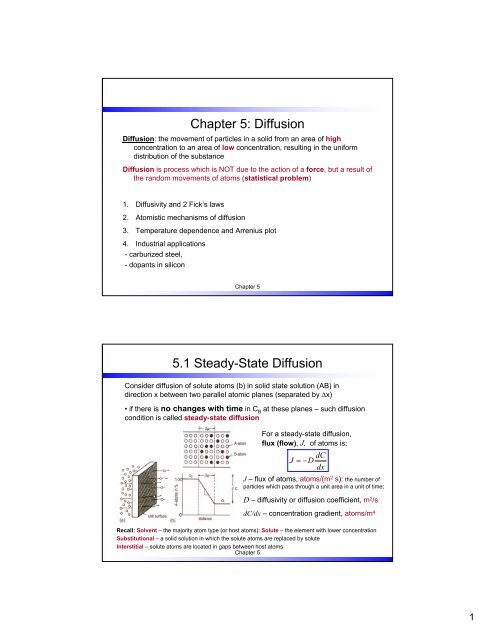
Chapter 5: Diffusion 5.1 Steady-State Diffusion

Chapter 5: Diffusion
Diffusion: the movement of particles in a solid from an area of high
concentration to an area of low concentration, resulting in the uniform
distribution of the substance
Diffusion is process which is NOT due to the action of a force, but a result of
the random movements of atoms (statistical problem)
1. Diffusivity and 2 Fick’s laws
2. Atomistic mechanisms of diffusion
3. Temperature dependence and Arrenius plot
4. Industrial applications
- carburized steel,
- dopants in silicon
Chapter 5
5.1 Steady-State Diffusion
Consider diffusion of solute atoms (b) in solid state solution (AB) in
direction x between two parallel atomic planes (separated by ∆x)
• if there is no changes with time in C B
at these planes – such diffusion
condition is called steady-state diffusion
For a steady-state diffusion,
flux (flow), J, of atoms is:
dC
J = −D
dx
J – flux of atoms, atoms/(m 2 s): the number of
particles which pass through a unit area in a unit of time;
D – diffusivity or diffusion coefficient, m 2 /s
dC/dx – concentration gradient, atoms/m 4
Recall: Solvent – the majority atom type (or host atoms): Solute – the element with lower concentration
Substitutional – a solid solution in which the solute atoms are replaced by solute
Interstitial – solute atoms are located in gaps between host atoms
Chapter 5
1

Fick’s first law of diffusion
dC
J = −D
dx
⎛ atoms ⎞ ⎛ m
J⎜
⎟ = −D
⎜
2
⎝ m s ⎠ ⎝ s
‘-’ sign: flux direction is from
the higher to the lower
concentration; i.e. it is the
opposite to the concentration
gradient
2
For steady-state diffusion condition (no change in the
system with time), the net flow of atoms is equal to the
diffusivity D times the diffusion gradient dC/dx
⎞ dC ⎛ atoms 1 ⎞
⎟ ⎜ ×
3
⎟
⎠ dx ⎝ m m ⎠
Diffusivity D depends on:
1. Diffusion mechanism
2. Temperature of diffusion
3. Type of crystal structure (bcc > fcc)
4. Crystal imperfections
5. Concentration of diffusing species
Chapter 5
Non-Steady-State Diffusion
In practice the concentration of solute atoms at any point in
the material changes with time – non-steady-state diffusion
For non-steady-state condition, diffusion
coefficient, D - NOT dependent on time:
Second Fick’s law of diffusion:
If D ≠ D(x), in 1D case:
dC
dt
x
=
dC x
dt
d
dx
⎛ dC
⎜ D
⎝ dx
2
∂ C
= D
2
∂x
x
⎞
⎟
⎠
Change in concentration in 2 semi-infinite
rods of Cu and Ni caused by diffusion, From
G. Gottstein “Physical Foundations of
Material Science”
The rate of compositional change is equal to
the diffusivity times the rate of the change of
the concentration gradient
In 3D case:
dC x
dt
2 2 2
⎛ ∂ C ∂ C ∂ C ⎞
D
⎜ + +
⎟
2 2
⎝ ∂x
∂y
∂z
⎠
=
2
Chapter 5
2

Non-Steady-State Diffusion (continued)
With specific initial or boundary conditions this partial differential equations can be solved
to give the concentration as function of spatial position and time c(x, y, z, t)
Let us consider two rods with different concentrations c 1
and c 2 which are joined at x=0 and both are so long that
mathematically they can be considered as infinitely long
The concentration profile at t = 0 is discontinuous at x = 0:
x < 0, c = c 1 ; x < 0, c = c 2
2
dC
We can obtain solution of: x
∂ C
= D
2
dt ∂x
c
c(
x,
t)
− c =
where erf ( z)
=
x
z =
2 Dt
1
2
− c
π
2
1
2
π
z
∫
0
x
Dt
∫
−∞
e
e
2
−ξ
2
−ξ
c
dξ
=
2
− c ⎛
1 ⎛ x ⎞⎞
1
2
⎜ + erf ⎜ ⎟
2
⎟
⎝ ⎝ Dt ⎠⎠
dξ,
is known as the error function
Chapter 5
Gas diffusion into a solid
Let us consider the case of a gas A diffusing into a solid B
Gas A
Solid B
Cs
− Cx
C − C
S
o
⎛
= erf ⎜
⎝ 2
x
Dt
⎞
⎟
⎠
x = 0
C S – surf. C of element in gas diffusing into the
surface
C o – initial uniform concentration of element in
solid
x - distance from surface
D – diffusivity of diffusing solute element
t – time
erf – mathematical function called error function
Chapter 5
3

Error function
Curve of the error function erf (z) for
z =
2
x
Dt
Chapter 5
Q: Consider the gas carburizing of a gear of 1018 steel (C 0.18 wt %) at 927°C. Calculate the time
necessary to increase the C content to 0.35 wt % at 0.40 mm below the surface of the gear. Assume the C
content at the surface to be 1.15 wt % and that the nominal C content of the steel gear before carburizing is
0.18 wt %. D (C in γ iron) at 927°C = 1.28 × 10 -11 m 2 /s
Chapter 5
4

5.2 Atomistics of Solid State Diffusion
• Diffusion mechanisms:
1. Vacancy (substitutional) diffusion – migration of atom in a lattice assisted
by the presence of vacancies
Ex.: self diffusion of Cu atoms in Cu crystal
2. Interstitial diffusion – movement of atoms from one interstitial site to
another neighboring interstitial site without permanent displacement any of
the atoms in the matrix crystal lattice
Ex.: C diffusion in BCC iron
Chapter 5
Vacancies
The simplest point defect is the vacancy (V) – an atom site from which an
atom is missing
Vacancies are always present; their number N V depends on temperature (T)
N
V
= N × e
EV
−
kT
N V - # of vacancies
N - number of lattice sites
E V – energy required to form a vacancy
k – Boltzmann constant
k = 1.38 ×10 -23 J K -1 ; or 8.62 ×10 -5 eV K -1
T – absolute temperature
vacancy
Chapter 5
5

Vacancy (Substitutional) Diffusion Mechanism
Substitutional (in homogeneous system - self-diffusion,
in heterogeneous system – solid state solutions)
• Vacancies are always present at any T
• As T increases ⇒ # of vacancies increases ⇒
diffusion rate increases
• Move atom A (from (1) to (2)) = move vacancy from
(2) to (1)..
higher T melt
⇒ stronger bonding between atoms ⇒ high activation energy to move V
Chapter 5
Kirkendall effect
• Marker at the diffusion interface move slightly in the opposite direction to the
most rapidly moving species ⇒ vacancies can move!
Chapter 5
6

Possible mechanisms of self-diffusion and their
activation energy
1. Neighboring atoms exchange sites
2. Ring mechanism
3. Vacancy mechanism
4. Direct interstitial mechanism
5. Indirect interstitial mechanism
Migration
Formation
Total
1
3
8 eV
1 eV
-
1 eV
8 eV
2 eV
4
0.6 eV
3.4 eV
4 eV
6
0.2 eV
3.4 eV
3.6 eV
Chapter 5
Anisotropy Effects
From G.Gottstein “Physical Foundations of Material Science”
Chapter 5
7

Carbon diffusion in Fe
Jump frequency Γ [s -1 ] of an atom is given by:
Γ = ν
kT
×e −G m
Usually ν≅10 13 [s -1 ] vibrational frequency of the atom
There is a fundamental relationship between the jump
frequency Γ and the diffusion coefficient D which is
independent of mechanism and crystal structure:
2
2
λ λ
D = ×Γ =
6 6τ
λ – the jump distance of the diffusing atom
τ =1/Γ – the time interval between two jumps
J = J MN
- J NM
A 1 2 A 1 2
J = C M
×Γ× × − CN
×Γ× ×
4 3 4 3
2
D =
Γa
24
Chapter 5
Carbon diffusion in Fe
Can be derived from an atomistic considerations of the
diffusion processes
C atoms are located on the octahedral interstitial sites
(black circles)
J = J MN
- J NM
Only ¼ of possible jumps of C atoms lead to flux in +x
Only 2/3 of all C atoms can jump in x direction
2
2
λ λ
D = ×Γ =
6 6τ
2
D =
Γa
24
Chapter 5
8

5.3 Effects of T on diffusion in solids
• Diffusion rate in a system will increase with temperature:
D = D × e
o
EA
−
RT
D – diffusivity, m 2 /s
D 0-
proportionality constant, m 2 /s, independent of T
E A – activation energy for diffusing species, J/mol
R – molar gas constant
R = 8.314 J mol-1 K-1; or 1.987cal mol-1K-1
T – absolute temperature
Chapter 5
Activation energy
A + B ⇒ C + D
A (initial state) ⇒ A* (final state)
• only a fraction of the molecules or atoms in a system will have
sufficient energy to reach E*
• A thermally active process is one which requires a definite amount
of thermal energy to overcome an activation energy barrier and enter
the reactive state
Chapter 5
9

Bolzmann’s equation
• On the basis of statistical analysis, Bolzmann’s results showed that the
probability of finding a molecule or atom at an energy level E * > the average
energy E of all the molecules or atoms in a system at a particular
temperature T, K, was:
Probability ∝ e
*
E −E
−
kT
where k B
= 1.38×10 -23 J/(atom K) -
Boltzmann’s constant
• The fraction of atoms or molecules in a system having energies > E* at a
given T (where E* is much greater than the average energy of any atom
or molecule:
n
N
total
= C × e
*
E
−
kT
Chapter 5
Arrhenius Rate Equation
The rate of many chemical reaction as a function of temperature as follows:
Rate _ of
_ reaction = C × e
E A
−
RT
C – rate constant, independent of T
E A – activation energy
R – molar gas constant
R = 8.314 J mol -1 K -1 ; or 1.987cal mol -1 K -1
T – absolute temperature
Chapter 5
10

If we rewrite in natural log plot:
EA
ln rate = ln C −
RT
ln rate = a
ln C = b
y = b + m×
x
1
x =
T
Typical Arrhenius Plot
or in logarithmic log plot:
log rate = log10
C
10
−
EA
2.303RT
Chapter 5
Q.: The diffusivity of Ag atoms in solid silver metal is 1.0X10 17 m 2 /s at 500 o C and 7.0x10 -13 m 2 /s at 1000 o C.
Calculate the activation energy (J/mole) for the diffusion of Ag in Ag in the T range 500 to 1000 o C.
Chapter 5
11

5.4 Industrial applications
Steel Hardening by Gas Carburizing
In the gas carburizing process for steel parts, the parts are placed in a
furnace in contact with a gas rich in CO-CH 4
mixture at ~927ºC.
Fe + x CH 4
⇒ FeC x
(x = 0.1-0.25% C), T = 927 o C
• The C from the gas diffuses into the surface of the steel part and
increases the C content of the outer surface region of the part.
• The higher C concentration at the surface makes the steel harder in
this region
• A steel part can thus be produced with a hard outer layer and a
tough low C steel inner core (important, for example, for many types
of gears)
Chapter 5
Dopants activation
Dopants can be incorporated into Si wafer to change their electrical conducting
characteristics
mask
Ion implantation
B, P + Annealing
Chapter 5
12

Q: If boron, B, is diffused into a thick slice of Si with no previous B in it at a temperature of 1100°C for 5 h,
what is the depth below the surface at which the concentration is 10 17 atoms/cm 3 if the surface concentration
is 10 18 atoms/cm3 D = 4 × 10 -13 cm 2 /s for B diffusing in Si at 1100°C.
Chapter 5
Summary
• Diffusion: the movement of particles in a solid from an area of high
concentration to an area of low concentration, resulting in the uniform
distribution of the substance
• Fick’s first diffusion law: for steady-state diffusion condition (no
change in the system with time), the net flow of atoms is equal to the
diffusivity D times the diffusion gradient dC/dx
J = −D
• Fick’s second diffusion law: The rate of compositional change is equal to
the diffusivity times the rate of the change of the concentration gradient
• Diffusion rate in a system will increase with temperature:
D = D × e
o
dC
dx
2
dC x
∂ C
= D
2
dt ∂x
EA
−
RT
Chapter 5
13