Algorithmic Differentiation in Python with Application Examples
Algorithmic Differentiation in Python with Application Examples
Algorithmic Differentiation in Python with Application Examples

Create successful ePaper yourself
Turn your PDF publications into a flip-book with our unique Google optimized e-Paper software.
<strong>Algorithmic</strong> <strong>Differentiation</strong> <strong>in</strong> <strong>Python</strong> <strong>with</strong><br />
<strong>Application</strong> <strong>Examples</strong><br />
Sebastian F. Walter, Humboldt-Universität zu Berl<strong>in</strong><br />
Wednesday, 10.07.2010<br />
Sebastian F. Walter, Humboldt-Universität zu Berl<strong>in</strong> <strong>Algorithmic</strong> () <strong>Differentiation</strong> <strong>in</strong> <strong>Python</strong> <strong>with</strong> <strong>Application</strong> <strong>Examples</strong>Wednesday, 10.07.2010 1 / 27
Part I: Intro to <strong>Algorithmic</strong> Diff.<br />
Comparison to Symbolic/Numerical <strong>Differentiation</strong><br />
The Forward Mode by Taylor Arithmetic<br />
The Reverse Mode<br />
Part II: Advanced <strong>Application</strong> <strong>Examples</strong><br />
<strong>Differentiation</strong> of Differential Equations<br />
<strong>Differentiation</strong> of Numerical L<strong>in</strong>ear Algebra Functions<br />
Optimum Experimental Design<br />
Standard Reference:<br />
Griewank, Evaluat<strong>in</strong>g Derivatives<br />
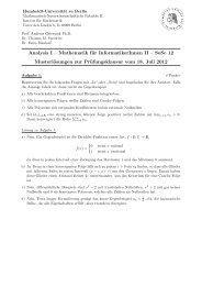
x(t; p)<br />
4<br />
3<br />
2<br />
1<br />
0<br />
−1<br />
−2<br />
−3<br />
−4<br />
0 1 2 3 4 5<br />
t<br />
10<br />
control func. u(t)<br />
8 state x(t)<br />
dx/dp1(t)<br />
6<br />
dx/dp2(t)<br />
x1(t; p = 1.0)<br />
x2(t; p = 1.0)<br />
dx1/dp(t; p = 1.0)<br />
dx2/dp(t; p = 1.0)<br />
h(t, x, p)<br />
dh/dp(t, x, p)<br />
d 2 x1/dp 2 (t; p = 1.0)<br />
d 2 x2/dp 2 (t; p = 1.0)<br />
state x(t)<br />
4<br />
2<br />
Research Community Website:<br />
www.autodiff.org<br />
0<br />
−2<br />
−4<br />
0.0 0.5 1.0 1.5 2.0 2.5 3.0 3.5 4.0<br />
time t [sec]<br />
Sebastian F. Walter, Humboldt-Universität zu Berl<strong>in</strong> <strong>Algorithmic</strong> () <strong>Differentiation</strong> <strong>in</strong> <strong>Python</strong> <strong>with</strong> <strong>Application</strong> <strong>Examples</strong>Wednesday, 10.07.2010 2 / 27
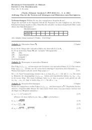
What is <strong>Algorithmic</strong> <strong>Differentiation</strong> (AD)<br />
Name confusion: <strong>Algorithmic</strong> <strong>Differentiation</strong> aka Automatic<br />
<strong>Differentiation</strong> aka Computational <strong>Differentiation</strong> aka AD<br />
Considered one of the most important algorithmic techniques “<strong>in</strong>vented”<br />
<strong>in</strong> the 20’th century 1<br />
Can be used to differentiate large-scale problems, e.g. <strong>in</strong> PDE<br />
constra<strong>in</strong>ed optimization.<br />
Generally much more efficient than symbolic/numerical differentiation<br />
and also accurate close to mach<strong>in</strong>e precision<br />
1 Nick Trefethen, http://www.comlab.ox.ac.uk/nick.trefethen/<strong>in</strong>ventorstalk.pdf<br />
Sebastian F. Walter, Humboldt-Universität zu Berl<strong>in</strong> <strong>Algorithmic</strong> () <strong>Differentiation</strong> <strong>in</strong> <strong>Python</strong> <strong>with</strong> <strong>Application</strong> <strong>Examples</strong>Wednesday, 10.07.2010 3 / 27
Software Used <strong>in</strong> this Talk:<br />
Name Description Status LOC<br />
algopy forward/reverse UTPM <strong>in</strong> <strong>Python</strong> alpha 10388<br />
www.github.com/b45ch1/algopy<br />
pysolv<strong>in</strong>d <strong>Python</strong> B<strong>in</strong>d<strong>in</strong>gs to SolvIND/DAESOL-II alpha 9743<br />
pyadolc <strong>Python</strong> B<strong>in</strong>d<strong>in</strong>gs to ADOL-C (C++) stable 6895<br />
www.github.com/b45ch1/pyadolc<br />
pycppad <strong>Python</strong> B<strong>in</strong>d<strong>in</strong>gs to CppAD (C++ ) stable 1334<br />
www.github.com/b45ch1/pycppad<br />
taylorpoly ANSI-C <strong>with</strong> <strong>Python</strong> b<strong>in</strong>d<strong>in</strong>gs alpha 9276<br />
www.github.com/b45ch1/taylorpoly<br />
easyodoe Opt. Exp. prototype alpha 8345<br />
Sebastian F. Walter, Humboldt-Universität zu Berl<strong>in</strong> <strong>Algorithmic</strong> () <strong>Differentiation</strong> <strong>in</strong> <strong>Python</strong> <strong>with</strong> <strong>Application</strong> <strong>Examples</strong>Wednesday, 10.07.2010 4 / 27
Why not Symbolic <strong>Differentiation</strong><br />
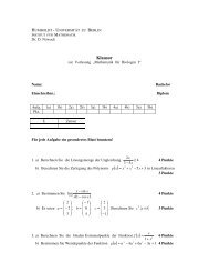
A Raytrac<strong>in</strong>g Example<br />
1.0<br />
0.5<br />
0.0 8<br />
6<br />
−0.5<br />
1<br />
3<br />
5<br />
7<br />
9<br />
Cyl<strong>in</strong>drical mirror described by 0 = g(x) = x 2 1 + x2 2 − 1,<br />
laser beam enters at x = (0, −1) and direction v.<br />
Recursive algorithm for next reflection po<strong>in</strong>t x + and<br />
direction v + :<br />
„ x +<br />
v + «<br />
0<br />
B<br />
= F(x, v) = @ x +<br />
r !<br />
“ ” x T 2<br />
v ‖x‖<br />
‖v‖ − 2 −1<br />
2 ‖v‖ 2 − xT v<br />
‖v‖ 2<br />
P(x + )v<br />
4<br />
2<br />
0<br />
−1.0<br />
−1.0 −0.5 0.0 0.5 1.0<br />
where P(x + ) = I − 2 wwT<br />
‖w‖ 2 , w = w(x + ) = ∇ xg(x + )<br />
Goal: compute sensitivity of the 10’th reflection po<strong>in</strong>t x (10) w.r.t. <strong>in</strong>itial<br />
direction v (0) , i.e. dx(10)<br />
dv (0) .<br />
Sebastian F. Walter, Humboldt-Universität zu Berl<strong>in</strong> <strong>Algorithmic</strong> () <strong>Differentiation</strong> <strong>in</strong> <strong>Python</strong> <strong>with</strong> <strong>Application</strong> <strong>Examples</strong>Wednesday, 10.07.2010 5 / 27
Why not Symbolic <strong>Differentiation</strong> (cont)<br />
Compute recursively x (k) , v (k) = F(x (k−1) , v (k−1) ) as symbolic<br />
expression<br />
Use sum,product and cha<strong>in</strong>rule to compute the wanted derivative<br />
Problem: Expression swell (show live example)<br />
import p y l a b ; import numpy ; from numpy import s q r t , dot , cos , s i n , pi , l i n<br />
import sympy ; from sympy import s q r t<br />
def F ( x , v ) :<br />
””” computes next r e f l e c t i o n p o i n t x and d i r e c t i o n v ”””<br />
c = d o t ( v , v )<br />
x2 = [ x [ 0 ] + v [ 0 ] ∗ ( s q r t ( ( d o t ( x , v ) / c )∗∗2 −( d o t ( x , x ) − 1 . ) / c)− d o t ( x , v ) / c ) ,<br />
x [ 1 ] + v [ 1 ] ∗ ( s q r t ( ( d o t ( x , v ) / c )∗∗2 −( d o t ( x , x ) − 1 . ) / c)− d o t ( x , v ) / c ) ]<br />
w = x2<br />
v2 = [ ( v [ 0 ] − 2∗ w[ 0 ] ∗ d o t (w, v ) / d o t (w,w) ) ,<br />
( v [ 1 ] − 2∗ w[ 1 ] ∗ d o t (w, v ) / d o t (w,w ) ) ]<br />
return x2 , v2<br />
x1 , x2 , v1 , v2 = sympy . symbols ( ’ x1 ’ , ’ x2 ’ , ’ v1 ’ , ’ v2 ’ )<br />
x = [ x1 , x2 ] ; v = [ v1 , v2 ]<br />
x , v = F ( x , v )<br />
p r i n t ’x , v=\n ’ , x , v<br />
#x , v = F ( x , v )<br />
Sebastian # p rF. i Walter, n t ’x Humboldt-Universität , v=\n ’ , x , v zu Berl<strong>in</strong> <strong>Algorithmic</strong> () <strong>Differentiation</strong> <strong>in</strong> <strong>Python</strong> <strong>with</strong> <strong>Application</strong> <strong>Examples</strong>Wednesday, 10.07.2010 6 / 27
Why not F<strong>in</strong>ite Differences<br />
Problem: F<strong>in</strong>ite Precision Arithmetic<br />
f (x) true value, ˜f (x) numerically computed value (assume x = ˜x)<br />
d˜f (x; v) = ˜f (x + tv) − ˜f (x)<br />
= f (x + tv) + δ 1 − f (x) + δ 2<br />
t<br />
t<br />
=<br />
f (x + tv) − f (x)<br />
+ δ 1 + δ 2<br />
t<br />
t<br />
=<br />
r(x; tv)<br />
df (x; v) − + δ 1 + δ 2<br />
,<br />
t t<br />
where δ 1 and δ 2 random errors due to f<strong>in</strong>ite precision arithmetic<br />
Difference numerical and true derivative:<br />
d˜f (x; v) − df (x; v) =<br />
r(x; tv)<br />
− δ 1 + δ 2<br />
,<br />
} {{<br />
t<br />
} } {{<br />
t<br />
}<br />
Question: What is the best t ∈ R<br />
t→0<br />
→ 0<br />
t→0<br />
→ ∞<br />
if f ∈ C 2 (R), then r(x; tv)/t = f ′′ (ξ)t and therefore t =<br />
√<br />
δ1 +δ 2<br />
f ′′ (ξ)<br />
Sebastian F. Walter, Humboldt-Universität zu Berl<strong>in</strong> <strong>Algorithmic</strong> () <strong>Differentiation</strong> <strong>in</strong> <strong>Python</strong> <strong>with</strong> <strong>Application</strong> <strong>Examples</strong>Wednesday, 10.07.2010 7 / 27
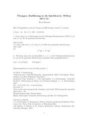
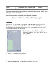
Why not F<strong>in</strong>ite Differences (cont.)<br />
absolute FD error<br />
10 33<br />
10 30<br />
10 27<br />
10 24<br />
10 21<br />
10 18<br />
10 15<br />
10 12<br />
10 9<br />
10 6<br />
10 3<br />
test function: f(x) = 1 + s<strong>in</strong>(x), x = 1<br />
FD 1st order<br />
FD 2nd order<br />
FD 3rd order<br />
10 0<br />
10 −3<br />
10 −6<br />
10 −9<br />
10 −16 10 −14 10 −12 10 −10 10 −8 10 −6 10 −4 10 −2 10 0<br />
step width t<br />
mach<strong>in</strong>e EPS ≈ 10 −16 for 64bit IEEE-754 floats<br />
higher-order derivatives by FD quickly get to large<br />
best t is not known a priory and often has to be guessed by careful tests<br />
Sebastian F. Walter, Humboldt-Universität zu Berl<strong>in</strong> <strong>Algorithmic</strong> () <strong>Differentiation</strong> <strong>in</strong> <strong>Python</strong> <strong>with</strong> <strong>Application</strong> <strong>Examples</strong>Wednesday, 10.07.2010 8 / 27
Part I:<br />
Intro <strong>Algorithmic</strong> <strong>Differentiation</strong><br />
Sebastian F. Walter, Humboldt-Universität zu Berl<strong>in</strong> <strong>Algorithmic</strong> () <strong>Differentiation</strong> <strong>in</strong> <strong>Python</strong> <strong>with</strong> <strong>Application</strong> <strong>Examples</strong>Wednesday, 10.07.2010 9 / 27
Computational Model and the Evaluation Trace<br />
All computer programs are a sequence of elementary functions<br />
φ l ∈ {+, −, ∗, /, s<strong>in</strong>, exp, . . . }<br />
Symbolic dependency is resolved at each elementary function:<br />
pushforward of numerical values v j≺l<br />
Example: Evaluate Function f (3, 7):<br />
f : R 2 → R<br />
x ↦→ y = f (x) = s<strong>in</strong>(x 1 +cos(x 2 )∗x 1 )<br />
Computational Graph:<br />
Computational Trace:<br />
1 Id<br />
<strong>in</strong>dependent v −1 = x 1 = 3<br />
<strong>in</strong>dependent v 0 = x 2 = 7<br />
v 1 = φ 1 (v 0 ) = cos(v 0 )<br />
2 cos<br />
v 2 = φ 2 (v 1 , v −1 ) = v 1 v −1<br />
v 3 = φ 3 (v −1 , v 2 ) = v −1 + v 2<br />
3 __mul__<br />
v 4 = φ 4 (v 3 ) = s<strong>in</strong>(v 3 )<br />
4 __add__<br />
5 s<strong>in</strong><br />
0 Id<br />
Sebastian F. Walter, Humboldt-Universität zu Berl<strong>in</strong> <strong>Algorithmic</strong> () <strong>Differentiation</strong> <strong>in</strong> <strong>Python</strong> <strong>with</strong> <strong>Application</strong> <strong>Examples</strong> Wednesday, 10.07.2010 10 / 27
Code Trac<strong>in</strong>g <strong>with</strong> PYADOLC and ALGOPY<br />
import a d o l c ; import a l gopy ; import numpy ; from numpy import s i n , cos ;<br />
def f ( x ) :<br />
return s i n ( x [ 0 ] + cos ( x [ 1 ] ) ∗ x [ 0 ] )<br />
a d o l c . t r a c e o n ( 1 )<br />
x = a d o l c . a d o u b l e ( [ 3 , 7 ] ) ; a d o l c . i n d e p e n d e n t ( x )<br />
y = f ( x )<br />
a d o l c . d e p e n d e n t ( y ) ; a d o l c . t r a c e o f f ( )<br />
a d o l c . t a p e t o l a t e x ( 1 , [ 3 , 7 ] , [ 0 . ] )<br />
cg = a l g o p y . CGraph ( )<br />
x = [ a l g o p y . F u n c t i o n ( 3 . ) , a l g o p y . F u n c t i o n ( 7 . ) ]<br />
y = f ( x )<br />
cg . t r a c e o f f ( )<br />
cg . i n d e p e n d e n t F u n c t i o n L i s t = [ x [ 0 ] , x [ 1 ] ] ; cg . d e p e n d e n t F u n c t i o n L i s t = [ y ]<br />
cg . p l o t ( ’ c g r a p h s i m p l e f u n c t i o n . svg ’ )<br />
code op loc loc loc loc double double value value val<br />
33 start of tape<br />
39 take stock op 2 0 3.000000e + 00 n<br />
1 assign <strong>in</strong>d 0 3.000000e + 00<br />
1 assign <strong>in</strong>d 1 7.000000e + 00<br />
20 cos op 1 3 2 7.000000e + 00 6.569866e −<br />
15 mult a a 2 0 3 7.539023e − 01 3.000000e +<br />
11 plus a a 0 3 4 3.000000e + 00 2.261707e +<br />
21 s<strong>in</strong> op 4 6 5 5.261707e + 00 5.221055e −<br />
2 assign dep 5<br />
0 death not 0 6 −8.528809e −<br />
Sebastian32 F. Walter, endHumboldt-Universität of tape<br />
zu Berl<strong>in</strong> <strong>Algorithmic</strong> () <strong>Differentiation</strong> <strong>in</strong> <strong>Python</strong> <strong>with</strong> <strong>Application</strong> <strong>Examples</strong> Wednesday, 10.07.2010 11 / 27
PART I.1:<br />
The Forward Mode of AD by<br />
Univariate Taylor Polynomial (UTP) Arithmetic<br />
Sebastian F. Walter, Humboldt-Universität zu Berl<strong>in</strong> <strong>Algorithmic</strong> () <strong>Differentiation</strong> <strong>in</strong> <strong>Python</strong> <strong>with</strong> <strong>Application</strong> <strong>Examples</strong> Wednesday, 10.07.2010 12 / 27
Univariate Taylor Polynomial Arithmetic (UTP)<br />
Basic Observation 1: Let f : R N → R, then<br />
d<br />
dt f (x + e it)<br />
∣ = (∇ x f (x)) T · e i = ∂f<br />
t=0<br />
∂x i<br />
Basic Observation 2: Hessian<br />
d 2<br />
f (x + e i t 1 + e j t 2 ) ∣<br />
dt 1 dt 2<br />
∣<br />
t1 =t 2 =0<br />
= e T i ∇ 2 xf (x)e j = ∂2 f<br />
∂x i ∂x j<br />
e i = (0, . . . , 1, . . . , 0) is the i’th cartesian basis vector.<br />
Sebastian F. Walter, Humboldt-Universität zu Berl<strong>in</strong> <strong>Algorithmic</strong> () <strong>Differentiation</strong> <strong>in</strong> <strong>Python</strong> <strong>with</strong> <strong>Application</strong> <strong>Examples</strong> Wednesday, 10.07.2010 13 / 27
Univariate Taylor Polynomial Arithmetic (UTP) (cont.)<br />
Problem can be formulated as arithmetic on univariate Taylor<br />
polynomials (UTP)<br />
D−1<br />
∑<br />
[x] D = [x 0 , . . . , x D−1 ] = x d T d ∈ R(T)/(T D ) ,<br />
d=0<br />
T is an <strong>in</strong>determ<strong>in</strong>ate, i.e. a formal parameter<br />
x d ∈ R is called Taylor coefficient<br />
Def<strong>in</strong>e extension of Functions f : R → R, y = f (x):<br />
E D (f ) : R[T]/(T D ) → R[T]/(T D )<br />
[x] D ↦→ [y] D := ∑ 1 d d D−1<br />
d! dt d f ( ∑<br />
x d t d )<br />
T d ,<br />
∣<br />
d=0<br />
k=0<br />
} {{ t=0<br />
}<br />
≡y d<br />
Sebastian F. Walter, Humboldt-Universität zu Berl<strong>in</strong> <strong>Algorithmic</strong> () <strong>Differentiation</strong> <strong>in</strong> <strong>Python</strong> <strong>with</strong> <strong>Application</strong> <strong>Examples</strong> Wednesday, 10.07.2010 14 / 27
Univariate Taylor Polynomial Arithmetic (UTP) (cont.)<br />
Let f (x) = (h ◦ g)(x) = h(g(x)) be a composite function, then<br />
E D (f ) = E D (h) ◦ E D (g) .<br />
I.e. E D is a homomorphism that preserves the function composition.<br />
Therefore: Need algorithms to compute<br />
[y 0 , . . . , y D−1 ] = E D (φ)([x 0 , . . . , x D−1 ])<br />
only for the elementary functions φ ∈ {+, −, ∗, /, . . . } !<br />
Suggests implementation by function and operator overload<strong>in</strong>g, i.e.<br />
univariate Taylor polynomial (UTP) arithmetic.<br />
Sebastian F. Walter, Humboldt-Universität zu Berl<strong>in</strong> <strong>Algorithmic</strong> () <strong>Differentiation</strong> <strong>in</strong> <strong>Python</strong> <strong>with</strong> <strong>Application</strong> <strong>Examples</strong> Wednesday, 10.07.2010 15 / 27
Algorithms for Univariate Taylor Polynomials over Scalars (UTPS)<br />
b<strong>in</strong>ary operations<br />
unary operations<br />
z = φ(x, y) d = 0, . . . , D OPS MOVES<br />
x + cy z d = x d + cy d 2D 3D<br />
x × y z d = P d<br />
k=0 h<br />
x ky d−k D 2 3D<br />
x/y z d = 1 x y d − P i<br />
d−1<br />
0 k=0 z ky d−k D 2 3D<br />
y = φ(x) d = 0, . . . , D OPS MOVES<br />
h<br />
ln(x) ỹ d = 1 ˜x x d − P i<br />
d−1<br />
0 k=1 x d−kỹ k D 2 2D<br />
exp(x) ỹ d = P d<br />
k=1 y d−k˜x k D 2 2D<br />
√ h<br />
x yd = 1 x 2y d − P i<br />
d−1<br />
0 k=1 y 1<br />
ky d−k 2 D2 3D<br />
h<br />
x r ỹ d = 1 r P d<br />
x 0 k=1 y d−k˜x k − P i<br />
d−1<br />
k=1 x d−kỹ k 2D 2 2D<br />
s<strong>in</strong>(v) ˜s d = P d<br />
j=1 ṽjc d−j 2D 2 3D<br />
cos(v) ˜c d = P d<br />
j=1 −ṽ js d−j<br />
tan(v) ˜φd = P d<br />
j=1 w d−jṽ j<br />
˜w d = 2 P d<br />
j=1 φ d−j “<br />
˜φ j<br />
arcs<strong>in</strong>(v) ˜φd = w −1<br />
0 ṽ d − P d−1<br />
j=1 w d−j ˜φ<br />
”<br />
j<br />
˜w d = − P d<br />
j=1 v d−j “<br />
˜φ j<br />
arctan(v) ˜φd = w −1<br />
0 ṽ d − P d−1<br />
j=1 w d−j ˜φ<br />
”<br />
j<br />
˜w d = 2 P d<br />
j=1 v d−jṽ j<br />
Sebastian F. Walter, Humboldt-Universität zu Berl<strong>in</strong> <strong>Algorithmic</strong> () <strong>Differentiation</strong> <strong>in</strong> <strong>Python</strong> <strong>with</strong> <strong>Application</strong> <strong>Examples</strong> Wednesday, 10.07.2010 16 / 27
Live Example: Directional Derivatives us<strong>in</strong>g TAYLORPOLY<br />
Interpretation: extract derivatives from Taylor coefficients<br />
if [x] D = [x 0 , 1, 0, 0, . . . , 0], then<br />
y d = 1 d d D−1<br />
d! dt d f ( ∑<br />
x d t d )<br />
= dd f<br />
∣ dx d (x 0)1 ,<br />
t=0<br />
Example: f : R 2 → R<br />
k=0<br />
x ↦→ y = f (x) = s<strong>in</strong>(x 1 + cos(x 2 )x 1 )<br />
(( ) ( )∣<br />
Compute df<br />
dx 1<br />
(3, 7) = d 3 1 ∣∣∣t=0<br />
dt f + t<br />
7 0)<br />
import numpy ; from numpy import s i n , cos ; from t a y l o r p o l y import UTPS<br />
def f ( x ) :<br />
return s i n ( x [ 0 ] + cos ( x [ 1 ] ) ∗ x [ 0 ] ) + x [ 1 ] ∗ x [ 0 ]<br />
x = [ UTPS ( [ 3 , 1 ] ) , UTPS ( [ 7 , 0 ] ) ]<br />
y = f ( x )<br />
p r i n t ’ normal f u n c t i o n e v a l u a t i o n y 0 = f ( x 0 ) = ’ , y . d a t a [ 0 ]<br />
p r i n t ’ g r a d i e n t e v a l u a t i o n df / dx 1 = ’ , y . d a t a [ 1 ]<br />
Sebastian F. Walter, Humboldt-Universität zu Berl<strong>in</strong> <strong>Algorithmic</strong> () <strong>Differentiation</strong> <strong>in</strong> <strong>Python</strong> <strong>with</strong> <strong>Application</strong> <strong>Examples</strong> Wednesday, 10.07.2010 17 / 27
PART I.2:<br />
The Reverse Mode of AD<br />
Sebastian F. Walter, Humboldt-Universität zu Berl<strong>in</strong> <strong>Algorithmic</strong> () <strong>Differentiation</strong> <strong>in</strong> <strong>Python</strong> <strong>with</strong> <strong>Application</strong> <strong>Examples</strong> Wednesday, 10.07.2010 18 / 27
The Reverse Mode by Hand:<br />
Recall: y = f (x) = s<strong>in</strong>(x 1 + cos(x 2 )x 1 )<br />
<strong>in</strong>dependent v −1 = x 1 = 3<br />
<strong>in</strong>dependent v 0 = x 2 = 7<br />
v 1 = φ 1 (v 0 ) = cos(v 0 )<br />
v 2 = φ 2 (v 1 , v −1 ) = v 1 v −1<br />
v 3 = φ 3 (v −1 , v 2 ) = v −1 + v 2<br />
v 4 = φ 4 (v 3 ) = s<strong>in</strong>(v 3 )<br />
dependent y = v 4<br />
Reverse Mode by Hand: Successive Pullbacks<br />
dy = dφ 4 (v 3 ) = ∂φ 4(z)<br />
∂z<br />
˛ dv 3 = cos(v 3 )<br />
˛z=v3<br />
= ¯v 3 dφ 3 (v −1 , v 2 ) = ¯v 3 dv −1 + ¯v 3<br />
|{z} |{z}<br />
=¯v −1<br />
= (¯v −1 + ¯v 2 v 1 ) dv −1 + ¯v 2 v −1 dv 1<br />
| {z } | {z }<br />
=¯v −1<br />
=¯v 1<br />
= ¯v −1 dv −1 + (−¯v 1 s<strong>in</strong>(v 0 )) dv 0<br />
| {z }<br />
=¯v 0<br />
Interpretation: ¯v −1 ≡ df and ¯v dx 0 ≡ df<br />
1 dx 2<br />
Need to store v 0 , v 1 , v 3 , v 4 for the reverse mode!<br />
dv 3<br />
| {z }<br />
=¯v 3<br />
=¯v 2<br />
dv 2<br />
Sebastian F. Walter, Humboldt-Universität zu Berl<strong>in</strong> <strong>Algorithmic</strong> () <strong>Differentiation</strong> <strong>in</strong> <strong>Python</strong> <strong>with</strong> <strong>Application</strong> <strong>Examples</strong> Wednesday, 10.07.2010 19 / 27
Semi-Automatic Forward/Reverse Mode by Manual Trac<strong>in</strong>g<br />
import numpy ; from numpy import s i n , cos ; from t a y l o r p o l y import UTPS<br />
x1 = UTPS ( [ 3 , 1 , 0 ] , P = 2 ) ; x2 = UTPS ( [ 7 , 0 , 1 ] , P=2)<br />
# forward mode<br />
vm1 = x1 ; v0 = x2<br />
v1 = cos ( v0 )<br />
v2 = v1 ∗ vm1<br />
v3 = vm1 + v2<br />
y = v4 = s i n ( v3 )<br />
# r e v e r s e mode<br />
v4bar = UTPS ( [ 0 , 0 , 0 ] , P = 2 ) ; v3bar = UTPS ( [ 0 , 0 , 0 ] , P=2)<br />
v2bar = UTPS ( [ 0 , 0 , 0 ] , P = 2 ) ; v1bar = UTPS ( [ 0 , 0 , 0 ] , P=2)<br />
v0bar = UTPS ( [ 0 , 0 , 0 ] , P = 2 ) ; vm1bar = UTPS ( [ 0 , 0 , 0 ] , P=2)<br />
v4bar . d a t a [ 0 ] = 1 .<br />
v3bar += v4bar ∗ cos ( v3 )<br />
vm1bar += v3bar ; v2bar += v3bar<br />
v1bar += v2bar ∗ vm1 ; vm1bar += v2bar ∗ v1<br />
v0bar −= v1bar ∗ s i n ( v0 )<br />
g1 = y . d a t a [ 1 : ] ; g2 = numpy . a r r a y ( [ vm1bar . d a t a [ 0 ] , v0bar . d a t a [ 0 ] ] )<br />
p r i n t ’ f o r w a r d g r a d i e n t g ( x 0 )=\ n ’ , g1 , ’\ n r e v e r s e g r a d i e n t g ( x 0 )=\ n ’ , g2<br />
p r i n t ’ H e s s i a n H( x 0 )=\ n ’ , numpy . v s t a c k ( [ vm1bar . d a t a [ 1 : ] , v0bar . d a t a [ 1 : ] ] )<br />
can automatize this us<strong>in</strong>g a code tracer or source code transformation,<br />
e.g. <strong>with</strong> PYADOLC or ALGOPY<br />
Sebastian F. Walter, Humboldt-Universität zu Berl<strong>in</strong> <strong>Algorithmic</strong> () <strong>Differentiation</strong> <strong>in</strong> <strong>Python</strong> <strong>with</strong> <strong>Application</strong> <strong>Examples</strong> Wednesday, 10.07.2010 20 / 27
Forward Mode vs Reverse Mode<br />
Task: compute Jacobian J = dF<br />
dx for F : RN → R M<br />
Forward Mode:<br />
J = dF<br />
dx · S ,<br />
where S = I ∈ R N×N .<br />
Reverse Mode:<br />
J = ¯S T · dF<br />
dx ,<br />
where ¯S ∈ R M×M .<br />
Gradient: The number of arithmetic operations (OPS) for the gradient<br />
evaluation ∇f (x) ∈ R N is only a small constant multiple of the OPS for<br />
the function f itself.<br />
Example: If f : R 2500 → R and runtime(f )=30 sec then SD/FD would<br />
require about 2500 ∗ 30 sec ≈ 21 hours but only a couple of m<strong>in</strong>utes<br />
us<strong>in</strong>g AD<br />
Mode Operations Memory<br />
Forward ∝ N OPS(F) MEM(J) N MEM(F)<br />
Reverse ∝ M OPS(F) MEM(J) ∝ OPS(F)<br />
Sebastian F. Walter, Humboldt-Universität zu Berl<strong>in</strong> <strong>Algorithmic</strong> () <strong>Differentiation</strong> <strong>in</strong> <strong>Python</strong> <strong>with</strong> <strong>Application</strong> <strong>Examples</strong> Wednesday, 10.07.2010 21 / 27
M<strong>in</strong>imal Surface problem <strong>with</strong> PYADOLC<br />
Example where the Reverse Mode Excels<br />
(discretized) objective function:<br />
u : [0, 1] 2 → R , u ∈ C 1<br />
s<br />
Z 1 Z 1<br />
u ↦→<br />
1 +<br />
0 0<br />
≈<br />
m−1 X m−1 X<br />
O ij (u)<br />
„ « ∂u 2<br />
+<br />
∂x<br />
„ « ∂u 2<br />
∂y<br />
i=0 j=0<br />
"<br />
Õ ij (u) := h 2 1 + (u #<br />
i+1,j+1 − u i,j ) 2 + (u i,j+1 − u i+1,j ) 2<br />
4<br />
Nonl<strong>in</strong>ear Program <strong>with</strong> box constra<strong>in</strong>ts:<br />
u ∗ ∈ R m×m = argm<strong>in</strong> u Õ(u)<br />
therefore ∇ u Õ(u) ∈ R m×m , e.g. m = 50<br />
yields a gradient <strong>with</strong> 2500 elements ⇒ use<br />
reverse mode<br />
Sebastian F. Walter, Humboldt-Universität zu Berl<strong>in</strong> <strong>Algorithmic</strong> () <strong>Differentiation</strong> <strong>in</strong> <strong>Python</strong> <strong>with</strong> <strong>Application</strong> <strong>Examples</strong> Wednesday, 10.07.2010 22 / 27
A M<strong>in</strong>imal Surface Problem<br />
part of unit test of pyadolc: /pyadolc/tests/complicated tests.py<br />
import a d o l c ; import numpy ;<br />
def O t i l d e ( u ) :<br />
””” o b j e c t i v e f u n c t i o n of the m<strong>in</strong>imal s u r f a c e problem ”””<br />
M = numpy . shape ( u ) [ 0 ]<br />
h = 1 . / (M−1)<br />
return M∗∗2∗h∗∗2+numpy . sum ( 0 . 2 5 ∗ ( ( u [ 1 : , 1 : ] − u [0: −1 ,0: −1])∗∗2+( u [ 1 : , 0 : − 1<br />
M = 5 0 ; h = 1 . /M; u = numpy . z e r o s ( (M,M) , d t y p e = f l o a t )<br />
u [ 0 , : ] = [ numpy . s i n ( numpy . p i ∗ j ∗h / 2 . ) f o r j <strong>in</strong> r a n g e (M) ]<br />
u [ −1 ,:] = [ numpy . exp ( numpy . p i / 2 ) ∗ numpy . s i n ( numpy . p i ∗ j ∗ h / 2 . ) f o r j<br />
u [ : , 0 ] = 0<br />
u [: , −1]= [ numpy . exp ( i ∗h∗numpy . p i / 2 . ) f o r i <strong>in</strong> r a n g e (M) ]<br />
# t r a c e the o b j e c t i v e f u n c t i o n<br />
a d o l c . t r a c e o n ( 1 )<br />
au = a d o l c . a d o u b l e ( u )<br />
a d o l c . i n d e p e n d e n t ( au )<br />
ay = O t i l d e ( au )<br />
a d o l c . d e p e n d e n t ( ay )<br />
a d o l c . t r a c e o f f ( )<br />
# compute g r a d i e n t<br />
g AD = a d o l c . g r a d i e n t ( 1 , numpy . r a v e l ( u ) ) . r e s h a p e ( numpy . shape ( u ) )<br />
g AD [ : , 0 ] = 0 ; g AD [ 0 , : ] = 0 ; g AD [: , −1] = 0 ; g AD [ −1 ,:] = 0 # on the ed<br />
# compute dot ( Hessian , v ) , v random v e c t o r<br />
Hv AD = a d o l c . h e s s v e c ( 1 , numpy . r a v e l ( u ) , numpy . random . r and ( u . s i z e ) )<br />
Sebastian F. Walter, Humboldt-Universität zu Berl<strong>in</strong> <strong>Algorithmic</strong> () <strong>Differentiation</strong> <strong>in</strong> <strong>Python</strong> <strong>with</strong> <strong>Application</strong> <strong>Examples</strong> Wednesday, 10.07.2010 23 / 27
PART II:<br />
Advanced <strong>Application</strong>s <strong>Examples</strong><br />
Sebastian F. Walter, Humboldt-Universität zu Berl<strong>in</strong> <strong>Algorithmic</strong> () <strong>Differentiation</strong> <strong>in</strong> <strong>Python</strong> <strong>with</strong> <strong>Application</strong> <strong>Examples</strong> Wednesday, 10.07.2010 24 / 27
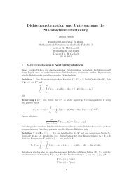
Optimum Experimental Design <strong>in</strong> Chemical Eng<strong>in</strong>eer<strong>in</strong>g<br />
Tetramethyl<br />
Cyclohexadien<br />
+<br />
k2 + Cat<br />
Pi−Complex +<br />
Cat<br />
λ<br />
Male<strong>in</strong>acid<br />
Anhydrid<br />
Male<strong>in</strong>acid<br />
Anhydrid<br />
Deactiv. Cat<br />
k1<br />
k3<br />
Diels−Alder<br />
Product<br />
− Cat<br />
non-catalyzed and catalyzed reaction path<br />
deactivation of the catalyst<br />
batch process<br />
measurements: product mass concentration<br />
control of educt molar numbers, catalyst<br />
concentration, temperature profile<br />
five unknown model parameters<br />
ṅ 1 = −k · n1 · n 2<br />
m tot<br />
, n 1 (0) = n a1<br />
ṅ 2 = −k · n1 · n 2<br />
m tot<br />
, n 2 (0) = n a2<br />
ṅ 3 = k · n1 · n 2<br />
m tot<br />
, n 3 (0) = 0<br />
k = k 1 · exp − E 1<br />
R ·<br />
1<br />
T − 1<br />
!!<br />
T ref<br />
+ k kat · c kat · exp (−λ · t) · exp − E kat<br />
R ·<br />
n 4 = n a4 T = ϑ + 273<br />
m tot = n 1 · M 1 + n 2 · M 2 + n 3 · M 3 + n 4 · M 4<br />
1<br />
T − 1<br />
!!<br />
T ref<br />
Sebastian F. Walter, Humboldt-Universität zu Berl<strong>in</strong> <strong>Algorithmic</strong> () <strong>Differentiation</strong> <strong>in</strong> <strong>Python</strong> <strong>with</strong> <strong>Application</strong> <strong>Examples</strong> Wednesday, 10.07.2010 25 / 27
Objective Function of Opt. Exp. Design<br />
Part I: Computation of J 1 and J 2<br />
J 1 [n mts, :] =<br />
√ wmts<br />
d<br />
(h(tnmts, x(tnmts; s, u(tnmts; q), p)))<br />
σ nmts (x(t nmts ; s, u(t nmts ; q), q) d(p, s)<br />
J 2 =<br />
d<br />
r(q, p, s)<br />
d(p, s)<br />
Part II: Numerical L<strong>in</strong>ear Algebra<br />
„<br />
J T<br />
C(J 1 , J 2 ) = (I, 0) 1 J 1 J2<br />
T « −1 „ « I<br />
J 2 0 0<br />
”<br />
=<br />
“Q T 2 (Q 2J1 T J 1Q T 2 )−1 Q 2<br />
Φ = λ 1 (C) , max. eigenvalue<br />
where J2 T = (QT 1 , QT 2 )(L, 0)T<br />
Computational Graph<br />
[p]<br />
[h], [r] [J 1 ], [J 2 ] [C] [Φ]<br />
[q]<br />
[s] [x 0 ] [x 1 ] [x 2 ] [x 3 ] [x 4 ] . . . [x N mts−1] [x N mts ]<br />
statex(t) atmeasurementtimes (mts)<br />
<strong>in</strong>dependent/dependent variables<br />
N mts Number measurement times, w measurement weight, σ std of a measurement, q controls, p nature<br />
Sebastian givenF. Walter, parameter, Humboldt-Universität s pseudo-Parameter zu Berl<strong>in</strong> <strong>Algorithmic</strong> ()(e.g. <strong>in</strong>itial <strong>Differentiation</strong> values), <strong>in</strong> u<strong>Python</strong> control <strong>with</strong> functions <strong>Application</strong> <strong>Examples</strong> Wednesday, 10.07.2010 26 / 27
Algorithm: Forward UTPM of the Rectangular QR Decomposition<br />
<strong>in</strong>put : [A] D = [A 0 , . . . , A D− 1], where A d ∈ R M×N , d = 0, . . . , D − 1, M ≥ N.<br />
output: [Q] D = [Q 0 , . . . , Q D− 1] matrix <strong>with</strong> orthonormal column vectors, where Q d ∈ R M×N ,<br />
d = 0, . . . , D − 1<br />
output: [R] D = [R 0 , . . . , R D− 1] upper triangular, where R d ∈ R N×N , d = 0, . . . , D − 1<br />
Q 0 , R 0 = qr (A 0 )<br />
for d = 1 to D − 1 do<br />
∆F = A d − P d−1<br />
k=1 Q d−kR k<br />
S = − 1 P d−1<br />
2 k=1 QT d−k Q k<br />
P L ◦ X = P L ◦ (Q T 0 ∆FR−1 0 − S)<br />
X = P L ◦ X − (P L ◦ X) T<br />
R d = Q T 0 ∆F − (S + X)R 0<br />
Q d = (∆F − Q 0 R d )R −1<br />
0<br />
end<br />
Sebastian F. Walter, Humboldt-Universität zu Berl<strong>in</strong> <strong>Algorithmic</strong> () <strong>Differentiation</strong> <strong>in</strong> <strong>Python</strong> <strong>with</strong> <strong>Application</strong> <strong>Examples</strong> Wednesday, 10.07.2010 27 / 27
Example for <strong>Differentiation</strong> of Numerical L<strong>in</strong>ear Algebra<br />
Compute directional derivatives of the largest eigenvalue,<br />
„<br />
J T<br />
∇ qλ max (I, 0) 1 J 1 J2<br />
T « −1 „ « ! I<br />
.<br />
J 2 0 0<br />
import numpy<br />
from a l g o p y import CGraph , F unction , UTPM, dot , <strong>in</strong>v , z e r o s , e i g h<br />
def P h i f c n (C ) :<br />
””” return max e i g e n v a l u e ”””<br />
return e i g h (C) [ 0 ] [ − 1 ]<br />
def Cfcn ( J1 , J2 ) :<br />
””” compute c o v a r i a n c e matrix ”””<br />
Np = J1 . shape [ 1 ] ; Nr = J2 . shape [ 0 ]<br />
tmp = z e r o s ( ( Np+Nr , Np+Nr ) , d t y p e =J1 )<br />
tmp [ : Np , : Np ] = d o t ( J1 . T , J1 )<br />
tmp [ Np : , : Np ] = J2<br />
tmp [ : Np , Np : ] = J2 . T<br />
return i n v ( tmp ) [ : Np , : Np ]<br />
D, P ,Nm, Np , Nr = 2 , 1 , 2 0 0 0 , 6 , 3<br />
cg = CGraph ( )<br />
J1 = F u n c t i o n (UTPM( numpy . random . r and (D, P ,Nm, Np ) ) )<br />
J2 = F u n c t i o n (UTPM( numpy . random . r and (D, P , Nr , Np ) ) )<br />
Phi = P h i f c n ( Cfcn ( J1 , J2 ) )<br />
cg . i n d e p e n d e n t F u n c t i o n L i s t = [ J1 , J2 ] ; cg . d e p e n d e n t F u n c t i o n L i s t = [ Phi ]<br />
p r i n t ’ o b j e c t i v e f u n c t i o n Phi =\n ’ , Phi<br />
Sebastian # cg F. . Walter, p l o t Humboldt-Universität ( ’ odoe cgraph zu Berl<strong>in</strong> . svg <strong>Algorithmic</strong> () ’ ) <strong>Differentiation</strong> <strong>in</strong> <strong>Python</strong> <strong>with</strong> <strong>Application</strong> <strong>Examples</strong> Wednesday, 10.07.2010 28 / 27
Sebastian F. Walter, Humboldt-Universität zu Berl<strong>in</strong> <strong>Algorithmic</strong> () <strong>Differentiation</strong> <strong>in</strong> <strong>Python</strong> <strong>with</strong> <strong>Application</strong> <strong>Examples</strong> Wednesday, 10.07.2010 29 / 27
Summary: Software Used <strong>in</strong> this Talk:<br />
Name Description Status LOC<br />
algopy forward/reverse UTPM <strong>in</strong> <strong>Python</strong> alpha 10388<br />
www.github.com/b45ch1/algopy<br />
pysolv<strong>in</strong>d <strong>Python</strong> B<strong>in</strong>d<strong>in</strong>gs to SolvIND/DAESOL-II alpha 9743<br />
pyadolc <strong>Python</strong> B<strong>in</strong>d<strong>in</strong>gs to ADOL-C (C++) stable 6895<br />
www.github.com/b45ch1/pyadolc<br />
pycppad <strong>Python</strong> B<strong>in</strong>d<strong>in</strong>gs to CppAD (C++ ) stable 1334<br />
www.github.com/b45ch1/pycppad<br />
taylorpoly ANSI-C <strong>with</strong> <strong>Python</strong> b<strong>in</strong>d<strong>in</strong>gs alpha 9276<br />
www.github.com/b45ch1/taylorpoly<br />
easyodoe Opt. Exp. prototype alpha 8345<br />
API is fairly well documented, about 30% of the LOCs<br />
quite complete unit test and many examples (<strong>in</strong>cluded <strong>in</strong> LOCs)<br />
ready to be used!<br />
Sebastian F. Walter, Humboldt-Universität zu Berl<strong>in</strong> <strong>Algorithmic</strong> () <strong>Differentiation</strong> <strong>in</strong> <strong>Python</strong> <strong>with</strong> <strong>Application</strong> <strong>Examples</strong> Wednesday, 10.07.2010 30 / 27