AD Tutorial at the TU Berlin

Not So Short Tutorial On 

Algorithmic Differentiation 

Sebastian F. Walter, HU Berlin 

Wednesday, 04.06.2010 

Sebastian F. Walter, HU Berlin () Not So Short Tutorial OnAlgorithmic Differentiation Wednesday, 04.06.2010 1 / 39

What is Algorithmic Differentiation? 

Name confusion: Algorithmic Differentiation aka Automatic 

Differentiation aka Computational Differentiation aka AD 

Considered one of the most important algorithmic techniques invented in 

the 20’th century 1 

Has distinct advantages over Finite Differences (FD) and Symbolic 

Differentiation (SD): more efficient and numerically stable and 

relatively easy to use. 

Can also be done by hand instead of symbolic differentiation (examples 

follow). 

1 Nick Trefethen, http://www.comlab.ox.ac.uk/nick.trefethen/inventorstalk.pdf 


Computational Model 

computer programs are a sequence of elementary functions 

φ l ∈ {+, −, ∗, /, sin, exp, . . . } 

Example: Evaluate Function f (3, 7): 

f : R 2 → R 

x ↦→ y = f (x) = sin(x 1 + cos(x 2 )x 1 ) 

Computational Trace: 

independent v −1 = x 1 = 3 

independent v 0 = x 2 = 7 

v 1 = φ 1 (v 0 ) = cos(v 0 ) 

v 2 = φ 2 (v 1 , v −1 ) = v 1 v −1 

v 3 = φ 3 (v −1 , v 2 ) = v −1 + v 2 

v 4 = φ 4 (v 3 ) = sin(v 3 ) 

dependent y = v 4 


Code Tracing with PYADOLC 

import numpy ; from numpy import s i n , cos ; import a d o l c 

def f ( x ) : 

return s i n ( x [ 0 ] + cos ( x [ 1 ] ) ∗ x [ 0 ] ) 

a d o l c . t r a c e o n ( 1 ) 

x = a d o l c . a d o u b l e ( [ 3 , 7 ] ) ; a d o l c . i n d e p e n d e n t ( x ) 

y = f ( x ) 

a d o l c . d e p e n d e n t ( y ) ; a d o l c . t r a c e o f f ( ) 

a d o l c . t a p e t o l a t e x ( 1 , [ 3 , 7 ] , [ 0 . ] ) 

code op loc loc loc loc double double value value val 

33 start of tape 

39 take stock op 2 0 3.000000e + 00 n 

1 assign ind 0 3.000000e + 00 

1 assign ind 1 7.000000e + 00 

20 cos op 1 3 2 7.000000e + 00 6.569866e − 

15 mult a a 2 0 3 7.539023e − 01 3.000000e + 

11 plus a a 0 3 4 3.000000e + 00 2.261707e + 

21 sin op 4 6 5 5.261707e + 00 5.221055e − 

2 assign dep 5 

0 death not 0 6 −8.528809e − 

32 end of tape 

All AD tools (implicitly) work on the computational trace. 


PART I: 

The Forward Mode of AD: Taylor Polynomial Arithmetic 


Algorithmic Differentiation ↔ Taylor Polynomial Arithmetic 

Basic Observation: Let f : R N → R, then 

d 

dt f (x + e nt) 

∣ = (∇ x f (x)) T · e n = ∂f , 

t=0 

∂x n 

where e n is the n’th cartesian basis vector. 

complete gradient can be obtained by taking e 1 , e 2 , . . . , e N 

for notational brevity: introduction of the seed matrix 

(∇ x f (x)) T · S = d dt f (x + St) ∣ 

∣∣∣t=0 

e.g. S = 

( 1 

1) 

S ∈ R N×P doesn’t have to be square and not necessarily be the identity 

matrix 

“using” a seed matrix also leads computationally more efficient 

algorithms (vectorized AD, e.g. adolc.hov forward) 


Univariate Taylor Polynomial Arithmetic (UTP) 

Notation for UTPs: 

D−1 

∑ 

[x] D := [x 0 , x 1 , . . . , x D−1 ] = x d T d ∈ R[T]/(T D ) , 

d=0 

T is an indeterminate, i.e. a formal parameter 

x d ∈ R is called Taylor coefficient 

a UTP is defined by the D coefficients x 0 , . . . , x D−1 

Definition of Functions on UTPs: 

E D (f ) : R[T]/(T D ) → R[T]/(T D ) 

[x] D ↦→ [y] D := ∑ 1 d d D−1 

d! dt d f ( ∑ 

x d t d ) 

T d , 

∣ 

d=0 

k=0 

} {{ t=0 

} 

≡y d 

where f : R → R, y = f (x) 

Required: algorithms to compute y d for the elem. funcs. +, −, ∗, /, . . . 


UTP of the Multiplication and Interpretation of UTP 

goal: compute [z] D = [x] D [y] D 

D−1 

∑ 

z d T d = 

d=0 

= 

D−1 

∑ 

D−1 

∑ 

x d T d y d T d 

d=0 

d=0 

D−1 

∑ d∑ 

( x d−k y k ) T d + O(T D ) 

d=0 k=0 

} {{ } 

=z d 

Interpretation: The coefficients y d of [y] D = E D (f )([x] D ) satisfy 

y d = dd f 

d d t (x 0 + 1t) ∣ 

∣ 

t=0 

= dd f 

d d x (x 0) 

if [x] D = [x 0 , 1, 0, . . . , 0] 

i.e. one gets higher-order derivatives by UTP arithmetic. 


Algorithms for Univariate Taylor Polynomials over Scalars (UTPS) 

binary operations 

unary operations 

z = φ(x, y) d = 0, . . . , D OPS MOVES 

x + cy z d = x d + cy d 2D 3D 

x × y z d = P d 

k=0 h 

x ky d−k D 2 3D 

x/y z d = 1 x y d − P i 

d−1 

0 k=0 z ky d−k D 2 3D 

y = φ(x) d = 0, . . . , D OPS MOVES 

h 

ln(x) ỹ d = 1 ˜x x d − P i 

d−1 

0 k=1 x d−kỹ k D 2 2D 

exp(x) ỹ d = P d 

k=1 y d−k˜x k D 2 2D 

√ h 

x yd = 1 x 2y d − P i 

d−1 

0 k=1 y 1 

ky d−k 2 D2 3D 

h 

x r ỹ d = 1 r P d 

x 0 k=1 y d−k˜x k − P i 

d−1 

k=1 x d−kỹ k 2D 2 2D 

sin(v) ˜s d = P d 

j=1 ṽjc d−j 2D 2 3D 

cos(v) ˜c d = P d 

j=1 −ṽ js d−j 

tan(v) ˜φd = P d 

j=1 w d−jṽ j 

˜w d = 2 P d 

j=1 φ d−j “ 

˜φ j 

arcsin(v) ˜φd = w −1 

0 ṽ d − P d−1 

j=1 w d−j ˜φ 

” 

j 

˜w d = − P d 

j=1 v d−j “ 

˜φ j 

arctan(v) ˜φd = w −1 

0 ṽ d − P d−1 

j=1 w d−j ˜φ 

” 

j 

˜w d = 2 P d 

j=1 v d−jṽ j 


Live Example: Gradient Evaluation using TAYLORPOLY 

Function: 

f : R 2 → R 

Compute Gradient∇ x f (3, 7) 

( ) 1 0 

seed matrix S = 

0 1 

x ↦→ y = f (x) = sin(x 1 + cos(x 2 )x 1 ) 

import numpy ; from numpy import s i n , cos ; from t a y l o r p o l y import UTPS 

def f ( x ) : 

return s i n ( x [ 0 ] + cos ( x [ 1 ] ) ∗ x [ 0 ] ) + x [ 1 ] ∗ x [ 0 ] 

x = [ UTPS ( [ 3 , 1 , 0 ] , P = 2 ) , UTPS ( [ 7 , 0 , 1 ] , P = 2 ) ] 

y = f ( x ) 

p r i n t ’ normal f u n c t i o n e v a l u a t i o n y 0 = f ( x 0 ) = ’ , y . d a t a [ 0 ] 

p r i n t ’ g r a d i e n t e v a l u a t i o n g ( x 0 ) = ’ , y . d a t a [ 1 : ] 


Higher-Order Mixed Partial Derivatives by UTP Arithmetic 

Always possible to compute higher-order mixed partial derivatives by 

evaluation/interpolation 2 

Example: Hessian H = [[f xx , f xy ], [f yx , f yy ]] 

〈s 1 |H|s 2 〉 = 1 2 [〈s 1|H|s 2 〉 + 〈s 2 |H|s 1 〉] 

= 1 2 [〈s 1 + s 2 − s 2 |H|s 2 〉 + 〈s 2 + s 1 − s 1 |H|s 1 〉] 

= 1 2 [〈s 1 + s 2 |H|s 1 + s 2 〉 − 〈s 1 |H|s 1 〉 − 〈s 2 |H|s 2 〉] . 

s T 1 ∇2 f (x)s 2 = ∂2 f (x + t 1 s 1 + t 2 s 2 ) 

∂t 1 ∂t 2 

˛˛˛˛t1 =t 2 =0 

= 1 » ∂ 2 – 

f (x + t(s 1 + s 2 )) 

2 ∂t 

˛˛˛˛t=0 2 − ∂2 f (x + s 1 t) 

∂t 2 − ∂2 f (x + s 2 t) 

∂t 2 . 

to get H ij use s 1 = e i and s 2 = e j cartesian basis vectors 

2 Griewank et al., Evaluating Higher Derivative Tensors by Forward Propagation of 

Univariate Taylor Series,Mathematics of Computation, 2000 


Live Example: Hessian Evaluation using TAYLORPOLY 

( ) 1 0 1 

f : R 2 → R, use seed matrix S = 

and propagate 

0 1 1 

( ( ) 

3 1 0 1 

[x] 3 = + 

T 

7) 

0 1 1 

from t a y l o r p o l y import UTPS 

def f f c n ( x ) : 

return s i n ( x [ 0 ] + cos ( x [ 1 ] ) ∗ x [ 0 ] ) 

S = a r r a y ( [ [ 1 , 0 , 1 ] , [ 0 , 1 , 1 ] ] , d t y p e = f l o a t ) 

P = S . shape [ 1 ] 

p r i n t ’ seed m a t r i x w ith P = %d d i r e c t i o n s S = \n ’%P , S 

x1 = UTPS ( z e r o s (1+2∗P ) , P = P ) 

x2 = UTPS ( z e r o s (1+2∗P ) , P = P ) 

x1 . d a t a [ 0 ] = 3 ; x1 . d a t a [ 1 : : 2 ] = S [ 0 , : ] 

x2 . d a t a [ 0 ] = 7 ; x2 . d a t a [ 1 : : 2 ] = S [ 1 , : ] 

y = f f c n ( [ x1 , x2 ] ) 

p r i n t ’ x1= ’ , x1 ; p r i n t ’ x2= ’ , x2 ; p r i n t ’ y= ’ , y 

H = z e r o s ( ( 2 , 2 ) , d t y p e = f l o a t ) 

H[ 0 , 0 ] = 2∗y . c o e f f [ 0 , 2 ] 

H[ 1 , 0 ] = H[ 0 , 1 ] = ( y . c o e f f [ 2 , 2 ] − y . c o e f f [ 0 , 2 ] − y . c o e f f [ 1 , 2 ] ) 

H[ 1 , 1 ] = 2∗y . c o e f f [ 1 , 2 ] 


PART II: 

The Reverse Mode of AD 


The Reverse Mode by Hand: 

Recall: y = f (x) = sin(x 1 + cos(x 2 )x 1 ) 

independent v −1 = x 1 = 3 

independent v 0 = x 2 = 7 

v 1 = φ 1 (v 0 ) = cos(v 0 ) 

v 2 = φ 2 (v 1 , v −1 ) = v 1 v −1 

v 3 = φ 3 (v −1 , v 2 ) = v −1 + v 2 

v 4 = φ 4 (v 3 ) = sin(v 3 ) 

dependent y = v 4 

Reverse Mode by Hand: Successive Pullbacks 

dy = dφ 4 (v 3 ) = ∂φ 4(z) 

∂z 

˛ dv 3 = cos(v 3 ) 

˛z=v3 

= ¯v 3 dφ 3 (v −1 , v 2 ) = ¯v 3 dv −1 + ¯v 3 

|{z} |{z} 

=¯v −1 

= (¯v −1 + ¯v 2 v 1 ) dv −1 + ¯v 2 v −1 dv 1 

| {z } | {z } 

=¯v −1 

=¯v 1 

= ¯v −1 dv −1 + (−¯v 1 sin(v 0 )) dv 0 

| {z } 

=¯v 0 

Interpretation: ¯v −1 ≡ df and ¯v dx 0 ≡ df 

1 dx 2 

Need to store v 0 , v 1 , v 3 , v 4 for the reverse mode! 

dv 3 

| {z } 

=¯v 3 

=¯v 2 

dv 2 


Live Example: Semi-Automatic Reverse Mode 


x1 = UTPS ( [ 3 , 1 , 0 ] , P = 2 ) ; x2 = UTPS ( [ 7 , 0 , 1 ] , P=2) 

# forward mode 

vm1 = x1 

v0 = x2 

v1 = cos ( v0 ) 

v2 = v1 ∗ vm1 

v3 = vm1 + v2 

v4 = s i n ( v3 ) 

y = v4 

# r e v e r s e mode 

v4bar = UTPS ( [ 0 , 0 , 0 ] , P = 2 ) ; v3bar = UTPS ( [ 0 , 0 , 0 ] , P=2) 

v2bar = UTPS ( [ 0 , 0 , 0 ] , P = 2 ) ; v1bar = UTPS ( [ 0 , 0 , 0 ] , P=2) 

v0bar = UTPS ( [ 0 , 0 , 0 ] , P = 2 ) ; vm1bar = UTPS ( [ 0 , 0 , 0 ] , P=2) 

v4bar . d a t a [ 0 ] = 1 . 

v3bar += v4bar ∗ cos ( v3 ) 

vm1bar += v3bar ; v2bar += v3bar 

v1bar += v2bar ∗ vm1 ; vm1bar += v2bar ∗ v1 

v0bar −= v1bar ∗ s i n ( v0 ) 

g1 = y . d a t a [ 1 : ] ; g2 = numpy . a r r a y ( [ vm1bar . d a t a [ 0 ] , v0bar . d a t a [ 0 ] ] ) 

p r i n t ’UTPS g r a d i e n t g ( x 0 )= ’ , g1 

p r i n t ’ r e v e r s e g r a d i e n t g ( x 0 )= ’ , g2 

p r i n t ’ H e s s i a n H( x 0 )=\ n ’ , numpy . v s t a c k ( [ vm1bar . d a t a [ 1 : ] , v0bar . d a t a [ 1 : ] ] ) 


Summary: Forward Mode and Reverse Mode 

Goal: compute Jacobian J = dF 

dx of function F : RN → R M 

Forward Mode: J = dF 

dx · S, where S = I ∈ RN×N 

needs N OPS(F) and MEM(J) ≤ N MEM(F) 

Reverse Mode: J = ¯S T · dF 

dx 

, where S = I ∈ RM×M 

OPS(J) ≈ M OPS(F) but MEM(J) ∼ OPS(F) 

Rule of Thumb: if 5M < N then reverse mode most likely more efficient, 

but only if and only if there is enough RAM! 

Partial Solution: can use Checkpointing to obtain logarithmic growth in 

the memory. 

For M ≪ N reverse mode will be the method of choice. 


PART III: 

Advanced AD and Applications 


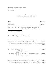
Optimum Experimental Design in Chemical Engineering 

Tetramethyl 

Cyclohexadien 

+ 

k2 + Cat 

Pi−Complex + 

Cat 

λ 

Maleinacid 

Anhydrid 

Maleinacid 

Anhydrid 

Deactiv. Cat 

k1 

k3 

Diels−Alder 

Product 

− Cat 

non-catalyzed and catalyzed reaction path 

deactivation of the catalyst 

batch process 

measurements: product mass concentration 

control of educt molar numbers, catalyst 

concentration, temperature profile 

five unknown model parameters 

ṅ 1 = −k · n1 · n 2 

m tot 

, n 1 (0) = n a1 

ṅ 2 = −k · n1 · n 2 

m tot 

, n 2 (0) = n a2 

ṅ 3 = k · n1 · n 2 

m tot 

, n 3 (0) = 0 

k = k 1 · exp − E 1 

R · 

1 

T − 1 

!! 

T ref 

+ k kat · c kat · exp (−λ · t) · exp − E kat 

R · 

n 4 = n a4 T = ϑ + 273 

m tot = n 1 · M 1 + n 2 · M 2 + n 3 · M 3 + n 4 · M 4 

1 

T − 1 

!! 

T ref 


Optimum Experimental Design in Chemical Engineering (Cont.) 

Dynamics: Defined by ODE 

Goal: Estimate parameters p = (k 1 , k kat , E kat ) 

Problem: Errors in the measurements η result in errors in parameters p. 

nonlinear regression with additive iid normal errors 

η m = h m(t m, x(t m), p, q) + ε m , 

ε m ∼ N (0, σ 2 m ) 

m = 1, . . . , N M 

η m are measurements, h measurement model function (connects model to the real world) 

Controls q = (n a1 , n a2 , n a4 , c kat , θ) influence the error propagation. 

Therefore: Find controls q such that the “uncertainty” in p is as “small” as possible. 

η 2 

ˆη(q 1 ) 

ˆη(q 2 ) 

J † (q) 

p 2 

ˆp(q 1 ) 

ˆp(q 2 ) 

Sebastian F. Walter, HU Berlin () Not So Short Tutorial OnAlgorithmic Differentiation Wednesday, 04.06.2010 19 / 39 

η 1 

p 1

Overall Objective Function 

Part I: Computation of J 1 and J 2 

J 1 [n mts, :] = 

√ wmts 

d 

σ nmts (x(t nmts ; s, u(t nmts ; q), q) d(p, s) (h(tnmts , x(t nmts ; s, u(t nmts ; q), p))) 

J 2 = 

d 

r(q, p, s) 

d(p, s) 

Part II: Numerical Linear Algebra 

„ 

J T 

C(J 1 , J 2 ) = (I, 0) 1 J 1 J2 

T « −1 „ « I 

J 2 0 0 

” 

= 

“Q T 2 (Q 2J1 T J 1Q T 2 )−1 Q 2 

where J2 T = (QT 1 , QT 2 )(L, 0)T 

Computational Graph 

[p] 

[h], [r] [J 1], [J 2] [C] [Φ] 

Φ = λ 1 (C) , max. eigenvalue 

[q] 

[s] [x 0] [x 1] [x 2] [x 3] [x 4] . . . [x Nmts−1] [xNmts ] 

statex(t) atmeasurementtimes (mts) independent/dependent variables 

N mts Number measurment times, σ std of a measurement, q controls, p nature given parameter, s 

pseudo-Parameter (e.g. initial values), u control functions 


Differentiation of ODE Solvers 

Explicit Euler: 

x k+1 = x k + h k f (t k , x k , p) 

want x(t) and dx 

dp (t) at t = [t 1, t 2 , . . . , t Nmts ] 

Idea: look at computation trace of the x k 

Apply Standard AD techniques + some tricks 

Approach also works for implicit schemes as needed for DAEs 

(DAESOL-II) 

[p] 

[h], [r] [J 1 ], [J 2 ] [C] [Φ] 

[q] 

[s] [x 0 ] [x 1 ] [x 2 ] [x 3 ] [x 4 ] . . . [x N mts−1] [x N mts ] 

statex(t) atmeasurementtimes (mts) 

independent/dependent variables 


Live Example: UTPS of Explicit Euler 


x = numpy . a r r a y ( [ UTPS ( [ 1 , 0 , 0 ] , P = 2 ) , UTPS ( [ 0 , 0 , 0 ] , P = 2 ) ] ) 

p = UTPS ( [ 3 , 1 , 0 ] , P=2) 

def f ( x ) : 

return numpy . a r r a y ( [ x [1] , − p ∗ x [ 0 ] ] ) 

t s = numpy . l i n s p a c e ( 0 , 2 ∗ numpy . pi , 1 0 0 ) 

x l i s t = [ [ x i . d a t a . copy ( ) f o r x i in x ] ] 

f o r n t s in r a n g e ( t s . s i z e −1): 

h = t s [ n t s +1] − t s [ n t s ] 

x = x + h ∗ f ( x ) 

x l i s t . append ( [ x i . d a t a . copy ( ) f o r x i in x ] ) 

xs = numpy . a r r a y ( x l i s t ) 

import m a t p l o t l i b . p y p l o t as p y p l o t 

p y p l o t . p l o t ( t s , xs [ : , 0 , 0 ] , ’ . k−’ , l a b e l = r ’ $x ( t ) $ ’ ) 

p y p l o t . p l o t ( t s , xs [ : , 0 , 1 ] , ’ . r−’ , l a b e l = r ’ $x p ( t ) $ ’ ) 

p y p l o t . x l a b e l ( ’ t ime $ t $ ’ ) 

p y p l o t . l e g e n d ( l o c = ’ b e s t ’ ) 

p y p l o t . g r i d ( ) 

p y p l o t . show ( ) 


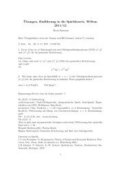
Application Example: DAESOL-II for Least-Squares 

2 

1 

0 

x(t; p) 

−1 

−2 

x 1 (t; p = 1.0) 

x 2 (t; p = 1.0) 

dx 1/dp(t; p = 1.0) 

dx 2 /dp(t; p = 1.0) 

η 1 

−3 

−4 

0 1 2 3 4 5 

t 

DAESOL-II can already do forward/reverse UTP 

UTP in DAESOL-II is approaching maturity now 

η 2 

x 1 (t; p = 1.6) 

x 2 (t; p = 1.6) 


Differentiating Implicitly Defined Function with Newton’s Method 

Many functions are implicitly defined by algebraic equations: 

multiplicative inverse: y = x −1 by 0 = xy − 1 

in general for independent x and dependent y: 

0 = F(x, y) 

Newton’s Method 3 : Let F([x], [y] D ) D = 0 and F ′ ([x], [y] D ) mod t D 

invertible. Then 

0 D+E = F([x], [y] D+E ) 

0 D+E = F([x], [y] D ) + F ′ ([x], [y] D )[∆y] E t D 

[∆y] E 

E = − 

( 

F ′ ([x], [y] E 

) −1 [∆F]E 

[X] D ≡ [X 0 , . . . , x D−1 ] ≡ ∑ D−1 

d=0 x dt d , [∆F] E t D D+E = F([x], [y] D ) 

if E = D then number of correct coefficients is doubled 

3 also called Newton-Hensel lifting or Hensel lifting 


Univariate Taylor Propagation on Matrices (UTPM) 

Application of Newton’s Method to defining equations 

Defining equations of the QR decomposition: 

0 

0 

0 

D 

= [Q] D [R] D − [A] D 

D 

= [Q] T D [Q] D − I 

D 

= P L ◦ [R] D , 

where (P L ) ij = δ i>j and element-wise multiplication ◦. 

Defining equations of the symmetric eigenvalue decomposition 

0 

0 

0 

D 

= [Q] T D [A] D[Q] D − [Λ] D 

D 

= [Q] T D [Q] D − I 

D 

= (P L + P R ) ◦ [Λ] D . 

Defining equations of the Cholesky Decomposition 

etc... 

0 

0 

0 

D 

= [L] D [L] T D − [a] D 

D 

= P D ◦ [L] D − I 

D 

= P R ◦ [L] D . 


Algorithm: Forward UTPM of the Rectangular QR Decomposition 

input : [A] D = [A 0 , . . . , A D− 1], where A d ∈ R M×N , d = 0, . . . , D − 1, M ≥ N. 

output: [Q] D = [Q 0 , . . . , Q D− 1] matrix with orthonormal column vectors, where Q d ∈ R M×N , 

d = 0, . . . , D − 1 

output: [R] D = [R 0 , . . . , R D− 1] upper triangular, where R d ∈ R N×N , d = 0, . . . , D − 1 

Q 0 , R 0 = qr (A 0 ) 

for d = 1 to D − 1 do 

∆F = A d − P d−1 

k=1 Q d−kR k 

S = − 1 P d−1 

2 k=1 QT d−k Q k 

P L ◦ X = P L ◦ (Q T 0 ∆FR−1 0 − S) 

X = P L ◦ X − (P L ◦ X) T 

R d = Q T 0 ∆F − (S + X)R 0 

Q d = (∆F − Q 0 R d )R −1 

0 

end 


Algorithm: Reverse UTPM of the Rectangular QR Decomposition 

input : [A] D = [A 0 , . . . , A D− 1], where A d ∈ R M×N , d = 0, . . . , D − 1, M ≥ N. 

output : [Q] D = [Q 0 , . . . , Q D− 1] matrix with orthonormal column vectors, where Q d ∈ R M×N , 

d = 0, . . . , D − 1 

output : [R] D = [R 0 , . . . , R D− 1] upper triangular, where R d ∈ R N×N , d = 0, . . . , D − 1 

input/output: [Ā] D = [Ā 0 , . . . , Ā D− 1], where Ā d ∈ R M×N , d = 0, . . . , D − 1, M ≥ N. 

input : [¯Q] D = [¯Q 0 , . . . , ¯Q D− 1], where ¯Q d ∈ R M×N , d = 0, . . . , D − 1 

input : [¯R] D = [¯R 0 , . . . , ¯R D− 1], where ¯R d ∈ R N×N , d = 0, . . . , D − 1 

[Ā] D = [Ā] D + ([¯Q] D − [Q] D [Q] T D [¯Q] D )[R] −T 

D ) 

+[Q] D 

“[¯R] D + P L ◦ `[R] D [¯R] T D − [¯R] D [R] T D + [Q]T D [¯Q] D − [¯Q] T D [Q] ´ ” 

D [R] 

−T 

D 


ALGOPY Live Example: QR decomposition 

import numpy ; from a l g o p y import UTPM 

# QR decomposition , UTPM forward 

D, P ,M,N = 3 , 1 , 5 , 2 

A = UTPM( numpy . random . rand (D, P ,M,N) ) 

Q, R = UTPM. qr (A) 

B = UTPM. d o t (Q, R) 

# check t h a t the r e s u l t s are c o r r e c t 

p r i n t ’Q. T Q − 1\n ’ ,UTPM. d o t (Q. T ,Q) − numpy . eye (N) 

p r i n t ’QR − A\n ’ ,B − A 

p r i n t ’ t r i u (R) − R\n ’ , UTPM. t r i u (R) − R 

# QR decomposition , UTPM r e v e r s e 

Bbar = UTPM( numpy . random . rand (D, P ,M,N) ) 

Qbar , Rbar = UTPM. p b d o t ( Bbar , Q, R , B) 

Abar = UTPM. p b q r ( Qbar , Rbar , A, Q, R) 

p r i n t 

’ Abar − Bbar \n ’ , Abar − Bbar 


ALGOPY Live Example: Moore-Penrose Pseudo inverse 

import numpy ; from algopy import CGraph , F unction , UTPM, dot , qr , eigh , in 

D, P ,M,N = 2 , 1 , 5 , 2 

# g e n e r a t e badly c o n d i t i o n e d matrix A 

A = UTPM( numpy . z e r o s ( ( D, P ,M,N ) ) ) 

x = UTPM( numpy . z e r o s ( ( D, P ,M, 1 ) ) ) ; y = UTPM( numpy . z e r o s ( ( D, P ,M, 1 ) ) ) 

x . d a t a [ 0 , 0 , : , 0 ] = [ 1 , 1 , 1 , 1 , 1 ] ; x . d a t a [ 1 , 0 , : , 0 ] = [ 1 , 1 , 1 , 1 , 1 ] 

y . d a t a [ 0 , 0 , : , 0 ] = [ 1 , 2 , 1 , 2 , 1 ] ; y . d a t a [ 1 , 0 , : , 0 ] = [ 1 , 2 , 1 , 2 , 1 ] 

a l p h a = 10∗∗−5; A = d o t ( x , x . T ) + a l p h a ∗ d o t ( y , y . T ) ; A = A [ : , : 2 ] 

# Method 1: Naive approach 

Apinv = d o t ( i n v ( d o t (A. T ,A) ) ,A. T ) 

p r i n t ’ n a i v e a p p r o a c h : A Apinv A − A = 0 \n ’ , d o t ( d o t (A, Apinv ) ,A) − A 

p r i n t ’ n a i v e a p p r o a c h : Apinv A Apinv − Apinv = 0 \n ’ , d o t ( d o t ( Apinv , A) , Ap 

p r i n t ’ n a i v e a p p r o a c h : ( Apinv A) ˆ T − Apinv A = 0 \n ’ , d o t ( Apinv , A ) . T − d 

p r i n t ’ n a i v e a p p r o a c h : (A Apinv ) ˆ T − A Apinv = 0 \n ’ , d o t (A, Apinv ) . T − d 

# Method 2: Using the d i f f e r e n t i a t e d QR decomposition 

Q, R = qr (A) 

tmp1 = s o l v e (R . T , A. T ) 

tmp2 = s o l v e (R , tmp1 ) 

Apinv = tmp2 

p r i n t ’QR a p p r o a c h : A Apinv A − A = 0 \n ’ , d o t ( d o t (A, Apinv ) ,A) − A 

p r i n t ’QR a p p r o a c h : Apinv A Apinv − Apinv = 0 \n ’ , d o t ( d o t ( Apinv , A) , Apinv 

p r i n t ’QR a p p r o a c h : ( Apinv A) ˆ T − Apinv A = 0 \n ’ , d o t ( Apinv , A ) . T − d o t ( 

p r i n t ’QR a p p r o a c h : (A Apinv ) ˆ T − A Apinv = 0 \n ’ , d o t (A, Apinv ) . T − d o t ( 


Algorithm: Forward UTPM of Symmetric Eigenvalue Decomposition 

input : [A] D = [A 0 , . . . , A D− 1], where A d ∈ R N×N symmetric positive definite, d = 0, . . . , D − 1 

output: [˜Λ] D = [˜Λ 0 , . . . , ˜Λ D− 1], where Λ 0 ∈ R N×N diagonal and Λ d ∈ R N×N block diagonal 

d = 1, . . . , D − 1. 

output: b ∈ N N b+1 , array of integers defining the blocks. The integer N B is the number of blocks. Each 

block has the size of the multiplicity of an eigenvalue λ nb of Λ 0 s.t. for sl = b[n b ] : b[n b + 1] one 

has (Q 0 [:, sl ]) T A 0 Q 0 [:, sl ] = λ nb I. 

Λ 0 , Q 0 = eigh (A 0 ) 

E ij = (Λ 0 ) jj − (Λ 0 ) ii 

H = P B ◦ (1/E) 

for d = 1 to D − 1 do 

S = − 1 2 

end 

P d−1 

k=1 QT d−k Q k 

K = ∆F + ˜Q T 0 A d ˜Q 0 + SΛ 0 + Λ 0 S 

˜Q d = Q 0 (S + H ◦ K) 

˜Λ d = ¯P B ◦ K 

for the special case of distinct eigenvalues, this algorithm suffices 

for repeated eigenvalues this algorithm is one step in a little more involved algorithm 


Test Example for the Symmetric Eigenvalue Decomposition 4 

Orthonormal Matrix: 

0 

1 

cos(x(t)) 1 sin(x(t)) −1 

1 

Q(t) = √ B− sin(x(t)) −1 cos(x(t)) −1 

C 

3 

@ 1 − sin(x(t)) 1 cos(x(t)) A 

−1 cos(x(t)) 1 sin(x(t)) 

Λ(t) = diag(x 2 − x + 1 2 , 4x2 − 3x, δ(− 1 2 x3 + 2x 2 − 3 2 x + 1) + (x3 + x 2 − 1), 3x − 1) , 

where x ≡ x(t) := 1 + t. 

constant δ = 0 means repeated eigenvalues, δ > 0 distinct but close 

In Taylor arithmetic one obtains 

Λ 0 = diag(1/2, 1, 1 + δ, 2) 

Λ 1 = diag(1, 5, 5 + δ, 3) 

Λ 2 = diag(2, 8, 8 + δ, 0) 

Λ 3 = diag(0, 0, 6 − 3δ, 0) 

Λ d = diag(0, 0, 0, 0), ∀d ≥ 4 . 

Define A(t) = Q(t)Λ(t)Q(t) and try to reconstruct Λ(t) and Q(t). 

4 Example adapted from Andrew and Tan, Computation of Derivatives of Repeated 

Eigenvalues and the Corresponding Eigenvectors of Symmetric Matrix Pencils, SIAM Journal 

on Matrix Analysis and Applications 


Test Example for the Symmetric Eigenvalue Decomposition (cont.) 

abs. error |λ 1 d − ˜λ 1 d | 

10 −14 

10 −15 

10 −16 

d = 0 

d = 1 

d = 2 

d = 3 

d = 4 

errors of λ 1 

10 −17 

10 −15 10 −14 10 −13 10 −12 10 −11 10 −10 10 −9 10 −8 10 −7 10 −6 10 −5 10 −4 10 −3 10 −2 10 −1 10 0 

δ 




10 −8 

10 −9 

10 −10 

10 −11 

10 −12 

10 −13 

10 −14 

10 −15 

errors of λ 2 d = 0 

d = 1 

d = 2 

d = 3 

d = 4 

10 −16 

10 −17 

10 −18 

10 −15 10 −14 10 −13 10 −12 10 −11 10 −10 10 −9 10 −8 10 −7 10 −6 10 −5 10 −4 10 −3 10 −2 10 −1 10 0 

δ 




10 −8 

10 −9 

10 −10 

10 −11 

10 −12 

10 −13 


d = 1 

d = 2 

d = 3 

d = 4 

10 −14 

10 −15 

10 −16 

10 −15 10 −14 10 −13 10 −12 10 −11 10 −10 10 −9 10 −8 10 −7 10 −6 10 −5 10 −4 10 −3 10 −2 10 −1 10 0 

δ 




10 −14 

10 −15 

10 −16 


d = 1 

d = 2 

d = 3 

d = 4 

10 −17 

10 −15 10 −14 10 −13 10 −12 10 −11 10 −10 10 −9 10 −8 10 −7 10 −6 10 −5 10 −4 10 −3 10 −2 10 −1 10 0 

δ 


The E-Criterion of the Opt. Exp. Design Problem 

Compute ∇ 2 qeigh(C(q)), where 

„ 

J T 

C = (I, 0) 1 J 1 J2 

T « −1 „ « I 

. 

J 2 0 0 

import numpy 

from a l g o p y import CGraph , F unction , UTPM; from a l g o p y . g l o b a l f u n c s import 

def C( J1 , J2 ) : 

Np = J1 . shape [ 1 ] ; Nr = J2 . shape [ 0 ] 

tmp = z e r o s ( ( Np+Nr , Np+Nr ) , d t y p e =J1 ) 

tmp [ : Np , : Np ] = d o t ( J1 . T , J1 ) 

tmp [ Np : , : Np ] = J2 

tmp [ : Np , Np : ] = J2 . T 

return i n v ( tmp ) [ : Np , : Np ] 

D, P ,Nm, Np , Nr = 2 , 1 , 5 0 , 4 , 3 

cg = CGraph ( ) 

J1 = F u n c t i o n (UTPM( numpy . random . r and (D, P ,Nm, Np ) ) ) 

J2 = F u n c t i o n (UTPM( numpy . random . r and (D, P , Nr , Np ) ) ) 

Phi = F u n c t i o n . e i g h (C( J1 , J2 ) ) [ 0 ] [ 0 ] 

cg . i n d e p e n d e n t F u n c t i o n L i s t = [ J1 , J2 ] ; cg . d e p e n d e n t F u n c t i o n L i s t = [ Phi ] 

cg . p l o t ( ’ p i c s / c g r a p h . svg ’ ) 



Some Software for Forward/Reverse UTP 

Name Description Status LOC 

algopy forward/reverse UTPM in Python alpha 10388 

www.github.com/b45ch1/algopy 

pysolvind Python Bindings to SolvIND/DAESOL-II alpha 9743 

pyadolc Python Bindings to ADOL-C (C++) stable 6895 

www.github.com/b45ch1/pyadolc 

pycppad Python Bindings to CppAD (C++ ) stable 1334 

www.github.com/b45ch1/pycppad 

taylorpoly ANSI-C with Python bindings alpha 9276 

www.github.com/b45ch1/taylorpoly 


Summary: 

Have shown many aspects of AD, in particular Univariate Taylor 

Polynomial arithmetic and the Reverse Mode 

There are many useful tools in Python that ease prototyping 

TAYLORPOLY hosts ANSI-C algorithms that can be used from basically 

all programming languages 

Outlook: 

Reverse mode of QR decomposition of quadratic by singular matrices 

Reverse mode of the symmetric eigenvalue decomposition for the case of 

repeated eigenvalues 

derive UTPM algorithm for the Singular Value Decomposition and 

generalized eigenvalue decomposition 

port all existing algorithms from ALGOPY to TAYLORPOLY

AD Tutorial at the TU Berlin

You also want an ePaper? Increase the reach of your titles

Delete template?

Save as template?