Advanced statistical analysis of epidemiological studies
Advanced statistical analysis of epidemiological studies
Advanced statistical analysis of epidemiological studies

You also want an ePaper? Increase the reach of your titles
YUMPU automatically turns print PDFs into web optimized ePapers that Google loves.
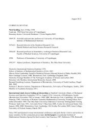
Ph.d. course in “<strong>Advanced</strong> <strong>statistical</strong><br />
<strong>analysis</strong> <strong>of</strong> <strong>epidemiological</strong> <strong>studies</strong>”<br />
Multi-state models, competing risks, recurrent events.<br />
Case-cohort <strong>studies</strong><br />
www.biostat.ku.dk/~pka/avepi11<br />
25 November 2011<br />
Per Kragh Andersen<br />
1
Multi-state models<br />
Survival data = cohort <strong>studies</strong> with a single outcome<br />
• time from “zero” to event (death)<br />
• right-censoring, delayed entry<br />
• basic quantity:<br />
– death intensity<br />
– = mortality rate<br />
– = hazard function<br />
– = h(t) ≈ Prob(die before t + ∆ | alive t)/∆<br />
<br />
✲<br />
0 t t + ∆<br />
2
Survival data.<br />
The hazard, h(t) provides a local (in time) description <strong>of</strong> the<br />
development.<br />
Models for h(t):<br />
• Cox regression<br />
• Poisson regression<br />
The survival function:<br />
S(t) = Prob(alive time t)<br />
describes the cumulative development over time.<br />
3
Two-state model for survival data<br />
0<br />
Alive<br />
h(t)<br />
✲<br />
1<br />
Dead<br />
h(t) ≈ Prob(state 1 time t + ∆ | state 0 time t)/∆<br />
S(t) = Prob(state 0 time t).<br />
F(t) = 1 − S(t) = Prob(state 1 time t) is the cumulative probability<br />
(“risk”) <strong>of</strong> death over the interval from 0 to t.<br />
4
Relation between rates and risks.<br />
We have the classical relation:<br />
S(t) = exp(−<br />
∫ t<br />
0<br />
h(u)du).<br />
This means that whenever we have a (Cox/Poisson/...) model for the<br />
rate, h(t), we also have a model for the risk: F(t) = 1 − S(t).<br />
In particular, if the rate increases/decreases with a covariate, Z, then<br />
also the risk increases/decreases with Z.<br />
5
Generalisations: competing risks<br />
0<br />
Dead, cause 1<br />
h 1 (t)<br />
✑ ✑✑✑✑✑✸<br />
♣<br />
Alive<br />
♣<br />
◗ ◗◗◗◗◗<br />
1<br />
h k (t)<br />
k<br />
Dead, cause k<br />
6
E.g., k = 3 causes:<br />
Competing risks<br />
• cancer<br />
• cardio-vascular diseases<br />
• other causes<br />
Cause-specific intensities (e.g. cause 1)<br />
h 1 (t) ≈ Prob(state 1 time t + ∆ | state 0 time t)/∆<br />
7
Generalisations: illness-death model<br />
0<br />
Disease-free<br />
h 01 (t)<br />
✲<br />
1<br />
Diseased<br />
❙<br />
❙<br />
❙<br />
❙✇<br />
h 02 (t)<br />
2<br />
Dead<br />
✓<br />
✓<br />
✓<br />
✓✴<br />
h 12 (t)<br />
The illness-death or disability model (chronic disease).<br />
8
Transition intensities<br />
Illness-death model<br />
“Disease incidence”:<br />
h 01 (t) ≈ Prob(state 1 time t + ∆ | state 0 time t)/∆<br />
Mortality among disease-free (e.g. standard mortality)<br />
h 02 (t) ≈ Prob(state 2 time t + ∆ | state 0 time t)/∆<br />
Mortality among diseased (“fatality rate”)<br />
h 12 (t) ≈ Prob(state 2 time t + ∆ | state 1 time t)/∆<br />
9
Generalisations: illness-death model<br />
0<br />
Disease-free<br />
❙<br />
❙<br />
❙<br />
❙✇<br />
h 02 (t)<br />
✛<br />
2<br />
h 01 (t)<br />
h 10 (t)<br />
Dead<br />
✲<br />
1<br />
Diseased<br />
✓<br />
✓<br />
✓<br />
✓✴<br />
h 12 (t)<br />
The illness-death or disability model (recurrent disease).<br />
10
Illness-death model, recurrent disease<br />
Transition intensities<br />
As above, but also “Cure rate”:<br />
h 10 (t) ≈ Prob(state 0 time t + ∆ | state 1 time t)/∆<br />
Also: Recurrent events, no death state.<br />
11
States:<br />
Bone marrow transplantations<br />
• Transplanted<br />
• Graft versus host disease<br />
• Relapse<br />
• Death<br />
etc. etc.<br />
12
Models are given by intensities:<br />
Common features<br />
h ij (t) ≈ Prob(state j time t + ∆ | state i time t)/∆<br />
Intensities may be modelled using:<br />
Cox regression, Poisson regression<br />
and analysed in SAS using<br />
PROC PHREG, PROC GENMOD<br />
In order to use PROC PHREG, a data file must be created for each<br />
transition including:<br />
• entry time (some times 0)<br />
• exit time<br />
• exit status (relevant transition or not)<br />
• covariates<br />
13
Common features<br />
In order to use PROC GENMOD, a data file must be created for each<br />
transition and for each combination <strong>of</strong> covariates, including:<br />
e.g.<br />
• time spent in state<br />
• number <strong>of</strong> transitions<br />
Age 1 Age 2 Age 3<br />
Exposed T 01 , D 01 T 02 , D 02 T 03 , D 03<br />
Non-exposed T 11 , D 11 T 12 , D 12 T 13 , D 13<br />
This enables us to analyse the intensities (rates) and estimate rate<br />
ratios<br />
14
Probabilities (risks)<br />
In survival <strong>analysis</strong>: The classical relation between risk and rate<br />
S(t) = exp(−<br />
∫ t<br />
0<br />
h(u)du).<br />
holds when there are no competing risks (e.g., C & H, ch. 4).<br />
In more general multi-state models:<br />
• transition probabilities are more complex functions <strong>of</strong> the<br />
intensities<br />
• few general computer programs exist<br />
(SAS MACRO for competing risks with “Cox hazards”, R packages<br />
cmprsk, mstate.)<br />
15
2 causes <strong>of</strong> death:<br />
In the competing risks model:<br />
P 00 (t) = Prob(alive time t)<br />
= exp(−<br />
∫ t<br />
0<br />
(h 1 (u) + h 2 (u))du).<br />
P 01 (t) = Prob(dead from cause 1 before time t) =<br />
∫ t<br />
0<br />
P 00 (u)h 1 (u)du<br />
<br />
0 u u + du t<br />
✲<br />
time<br />
16
This means that the cumulative incidence:<br />
P 01 (t) (and similarly P 02 (t))<br />
may be estimated from<br />
h 1 (t) and h 2 (t).<br />
That is, the risk for cause 1 depends on the rates for both causes 1<br />
and 2.<br />
The SE’s may also be estimated: a SAS MACRO and an R function are<br />
available.<br />
17
What does<br />
estimate<br />
In the competing risks model:<br />
1 − exp(−<br />
∫ t<br />
0<br />
h 1 (u)du)<br />
Prob(Dead from cause 1 before t)<br />
IF h 2 (t) = 0!<br />
i.e., if the competing risk does not exist.<br />
This hypothetical probability is rarely <strong>of</strong> interest. However, it is used<br />
frequently anyhow!<br />
“Relapse survival curve” in clinical cancer <strong>studies</strong>.<br />
“1-Kaplan-Meier” as risk estimator in <strong>epidemiological</strong> (and other)<br />
<strong>studies</strong>.<br />
18
Censoring in survival <strong>studies</strong><br />
Note that rates may be estimated by treating other events as<br />
censoring while risks require modeling <strong>of</strong> all competing events.<br />
When, in survival <strong>studies</strong>, we draw the Kaplan-Meier estimator only<br />
the death intensity is taken into account - NOT the censoring<br />
intensity. This makes sense if BOTH (I): the population without<br />
censoring makes sense, AND (II) censoring is “independent”.<br />
Example: event = death due to cancer, consider censoring due to<br />
• end <strong>of</strong> study<br />
• emigration, loss to follow-up<br />
• death due to traffic accidents<br />
• death due to cardiovascular disease<br />
Magnitude <strong>of</strong> (I) depends on magnitude <strong>of</strong> competing risk.<br />
19
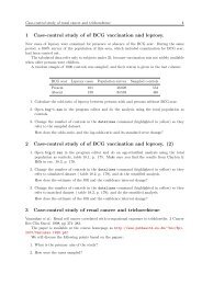
Competing risks example: bone marrow transplantation.<br />
1715 leukemia patients with BMT:<br />
• 537 ALL, 340 AML, 838 CML<br />
• 1026 early stage, 410 intermediate stage, 279 advanced stage<br />
• 1224 HLA-identical sibling, 383 HLA-matched unrelated donor,<br />
108 HLA-mismatched unrelated donor<br />
Analysis:<br />
• Cox regression models for cause-specific hazards <strong>of</strong> “relapse” and<br />
“death in remission”<br />
• Estimation <strong>of</strong> cumulative incidences<br />
20
Cox regression models for cause-specific hazards<br />
Relapse Death<br />
Covariate ˆβ (SD) ˆβ (SD)<br />
HLA-id. sibling 0 - 0 -<br />
HLA-matched donor 0.011 0.15 0.811 0.097<br />
HLA-mismatched donor -0.944 0.36 1.118 0.14<br />
ALL 0 - 0 -<br />
AML -0.271 0.15 -0.195 0.14<br />
CML -0.721 0.16 0.291 0.117<br />
Early stage 0 - 0 -<br />
Intermed. stage 0.640 0.15 0.474 0.10<br />
<strong>Advanced</strong> stage 1.848 0.15 0.781 0.13<br />
Karn<strong>of</strong>sky> 90 -0.118 0.14 -0.504 0.11<br />
21
Cumulative incidences<br />
22
Regression <strong>analysis</strong> <strong>of</strong> risks.<br />
The cumulative incidences may be related to covariates by fitting<br />
models for cause-specific hazards and plugging into the rate → risk<br />
relation. However, this does not give a simple relationship, e.g. a<br />
covariate may increase the rate <strong>of</strong> a given cause but decrease the<br />
corresponding risk depending on its effect on the other rates.<br />
Instead: direct modeling the relationship using the “Fine-Gray”<br />
model.<br />
Cox model for survival data: − log(1 − F(t)) = A 0 (t)e β′Z ,<br />
A 0 (t) cumulative baseline hazard.<br />
Fine-Gray model for P 01 (t): − log(1 − P 01 (t)) = A 01 (t)e β′ 1 Z .<br />
This gives a direct relationship between covariates and risk but the<br />
interpretation <strong>of</strong> the regression parameters, β 1 is not so simple.<br />
23
Fine-Gray regression models for cumulative incidences<br />
Relapse Death<br />
Covariate ˆβ1 (SD) ˆβ1 (SD)<br />
HLA-id. sibling 0 - 0 -<br />
HLA-matched donor -0.32 0.16 0.76 0.10<br />
HLA-mismatched donor -1.37 0.38 1.15 0.13<br />
ALL 0 - 0 -<br />
AML -0.17 0.15 -0.16 0.14<br />
CML -0.75 0.16 0.33 0.12<br />
Early stage 0 - 0 -<br />
Intermed. stage 0.51 0.15 0.41 0.10<br />
<strong>Advanced</strong> stage 1.51 0.15 0.45 0.13<br />
Karn<strong>of</strong>sky> 90 0.17 0.15 -0.44 0.11<br />
24
Recurrent events.<br />
Suppose individuals may experience the event recurrently, e.g.<br />
hospital admissions.<br />
Kessing, Olsen and Andersen, Amer. J. Epidemiol. (1999) studied<br />
data from Danish Central Psychiatric Registry, DCPR:<br />
• All psychiatric admissions 1 April 1970-<br />
• Discharge diagnoses<br />
• ICD-8 until 31 december 1993<br />
• ICD-10 from 1 January 1994<br />
and linked to the Danish Civil Registration System, ”CPR” to<br />
obtain information on vital status and emigration.<br />
25
Sample from register data.<br />
• All patients identified in DCPR before 1 January 1994 with a<br />
bipolar (“manic”) diagnosis at first discharge.<br />
• Restrict attention to patients younger than 52 years at diagnosis,<br />
1307 men and 1655 women.<br />
• Followed to 31 December 1999 w.r.t. later psychiatric<br />
admissions, death, diagnosis <strong>of</strong> schizophrenia or emigration.<br />
Purpose <strong>of</strong> study: Evaluate theory <strong>of</strong> “sensitization” (or “kindling”).<br />
According to this theory, mood episodes themselves stress the brain<br />
so that its sensitivity to biologic and psychosocial stressors increases.<br />
This leads to shorter and shorter intervals between successive<br />
episodes, e.g. (Post, 1992, Amer. J. Psych.)<br />
26
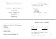
Register data.<br />
Kaplan-Meier estimates <strong>of</strong> the survivor functions<br />
for 1st, 2nd and later waiting times.<br />
Survival Function<br />
0.0 0.2 0.4 0.6 0.8 1.0<br />
Men<br />
1wt<br />
2wt<br />
3wt<br />
4wt<br />
5wt<br />
Survival Function<br />
0.0 0.2 0.4 0.6 0.8 1.0<br />
Women<br />
1wt<br />
2wt<br />
3wt<br />
4wt<br />
5wt<br />
0 1000 2000 3000 4000<br />
Time(days)<br />
0 1000 2000 3000 4000<br />
Time(days)<br />
27
Using Kaplan-Meier curves.<br />
The Kaplan-Meier curves do not properly address the problem <strong>of</strong><br />
sensitization due to selection/heterogeneity – those with 2 episodes is<br />
a select subgroup <strong>of</strong> those with 1 etc.<br />
Another way <strong>of</strong> stating the problem is via dependent censoring:<br />
e.g., censoring <strong>of</strong> the second waiting time depends on the first waiting<br />
time and if successive waiting times are correlated then censoring <strong>of</strong><br />
the second waiting time depends on the second waiting time:<br />
T i : duration <strong>of</strong> follow-up time for subject i, W i1 , W i2 : first and<br />
second waiting time for subject i.<br />
C i2 = T i − W i1 censoring time for W i2 . If W i1 and W i2 are dependent<br />
then W i2 and C i2 are also dependent.<br />
In the <strong>analysis</strong> we need to take this dependence into account.<br />
28
Random effects models.<br />
Random effects models for survival data are known as “frailty<br />
models”.<br />
Hazard function for waiting time no. j for patient no. i:<br />
h ij (t) = U i h 0 (t) exp(α j + β ′ Z i ).<br />
• U i : random “frailty” for patient i following some distribution<br />
with mean 1 and SD σ across the patient population<br />
• h 0 (t): baseline hazard<br />
• α j : log(hazard ratio) for waiting time no. j compared to<br />
reference waiting time (e.g. first waiting time)<br />
• Z i : covariates<br />
29
Results for younger bipolar patients.<br />
Men<br />
Women<br />
Episode (j) Rate ratio 95% c.i. Rate ratio 95% c.i.<br />
1 1.00 ref. 1.00 ref.<br />
2 1.18 1.03-1.34 1.22 1.08-1.37<br />
3 1.46 1.27-1.69 1.47 1.29-1.67<br />
4 1.72 1.49-2.02 1.61 1.40-1.85<br />
5+ 2.35 2.07-2.67 2.19 1.07-2.45<br />
σ 2 0 (no frailty) 0 (no frailty)<br />
1 1.00 ref. 1.00 ref.<br />
2 0.99 0.84-1.15 1.07 0.93-1.22<br />
3 1.10 0.91-1.33 1.16 0.99-1.36<br />
4 1.16 0.93-1.45 1.17 0.98-1.39<br />
5+ 1.30 1.04-1.64 1.25 1.04-1.50<br />
σ 2 0.45 0.26-0.63 0.41 0.28-0.54<br />
30
Study base: population followed from t 0 to t 1 .<br />
t 0 t 1<br />
<br />
<br />
❛<br />
<br />
❛ ❛<br />
♣<br />
❛<br />
31
Nested case-control study<br />
t 0 t 1<br />
❞<br />
❞<br />
❞<br />
❛<br />
❞<br />
❛<br />
❞<br />
❞<br />
❞<br />
❛ ❞ ❛<br />
♣<br />
❞<br />
32
Estimation <strong>of</strong> rate ratio θ:<br />
(<br />
)<br />
∑ θ (for case)<br />
log ∑<br />
failures<br />
Case-control set θ<br />
Compare: Cox regression in cohort study or matched case-control<br />
study.<br />
PROC PHREG in SAS may be used (but PROC LOGISTIC may be<br />
simpler).<br />
In the simplest case, the controls are a simple random sample from<br />
the risk set.<br />
33
Matching.<br />
Other nested case-control sampling designs.<br />
Example: Lung cancer incidence, smoking possible confounder.<br />
Many smoking cases, perhaps relatively few smoking controls ⇒<br />
random sampling <strong>of</strong> m − 1 controls will give few controls per smoking<br />
case and more controls per non-smoking case.<br />
Matching on smoking may be efficient.<br />
• Availability <strong>of</strong> data<br />
• Inability to estimate effect <strong>of</strong> smoking<br />
34
θ case = exp(β 1 · exposure case + β 2 · smoke case )<br />
θ control = exp(β 1 · exposure control + β 2 · smoke control )<br />
where exposure is 0 or 1 and and where the value <strong>of</strong> smoke is the<br />
same for case and controls, i.e. exp(β 2 ) cancels out in log partial<br />
likelihood:<br />
(<br />
)<br />
∑ θ (for case)<br />
log ∑<br />
failures<br />
Case-control set θ .<br />
35
Counter-matching.<br />
To do the matched study, the confounder must be known for every<br />
one.<br />
Suppose instead that exposure is known for every one but the<br />
confounder may be costly to obtain. Then:<br />
• Matching on exposure is possible, but disastrous!<br />
• Information on exposure may be used when selecting controls<br />
E.g. in a given risk set: N 1 = 10 exposed, N 0 = 100 non-exposed.<br />
Simple random sampling then leads to uneven (and inefficient)<br />
exposure distribution in sampled case-control set. Instead, let the<br />
case-control set consist <strong>of</strong> m = 5 + 1 = n 0 + n 1 = 3 + 3<br />
non-exposed/exposed individuals, i.e. if case is exposed then sample<br />
2 exposed + 3 non-exposed controls and if case is non-exposed then<br />
sample 3 exposed + 2 non-exposed controls.<br />
36
The confounder is ascertained for the sampled case-control set.<br />
In the log-likelihood: Members <strong>of</strong> the case-control sets must be<br />
weighted differently:<br />
(<br />
)<br />
∑ θ (for case)<br />
log ∑<br />
failures<br />
Case-control set w · θ .<br />
Here: w = N 1<br />
n 1<br />
= 10/3 for exposed<br />
w = N 0<br />
n 0<br />
= 100/3 for non-exposed<br />
“Counter-matching”: m − 1 = 1, case and control must have different<br />
exposure status.<br />
Counter-matching on surrogate exposure is also possible.<br />
Analysis: computer program must be able to deal with different<br />
weights: ‘‘OFFSET’’ in SAS PROC PHREG.<br />
37
Example <strong>of</strong> matched, nested c-c study.<br />
Josefson, Magnusson, Ylitalo, Sørensen, Qwarforth-Tubbin,<br />
Andersen, Melbye, Adami, Gyllensten Lancet, 2000, 355, 2189-93.<br />
• 146889 women screened between 1969 and 1995 in Uppsala<br />
county cervix cancer screening program: (732887 smears taken)<br />
• 478 cases <strong>of</strong> cervix cancer in situ (CIS) identified through the<br />
Swedish cancer register<br />
• 5 (potential) controls selected per case from the calendar time<br />
risk set, matched on time <strong>of</strong> entry into cohort (= time <strong>of</strong> first<br />
smear) and on age. NO matching on number <strong>of</strong> smears.<br />
• 1 <strong>of</strong> the 5 controls randomly selected for inclusion. If the selected<br />
control had only one smear then a second control was selected.<br />
(→ 608 controls.)<br />
38
• Exposure, HPV-16 viral load, ascertained from the 2081/1754<br />
available smears.<br />
Why do a nested case-control study<br />
• To avoid making cytological analyses <strong>of</strong> many smears.<br />
Why match<br />
• on age Standard, age is a confounder.<br />
• on time <strong>of</strong> first smear To make ”exposure quality” similar for<br />
cases and controls.<br />
39
Results.<br />
Josefsson et al., Lancet, 2000, 355, 2189-93.<br />
Viral load Cases/controls exp(β)<br />
HPV 16 negative 354/578 1<br />
Below 20 percentile 16/15 1.9 (0.8-4.2)<br />
20-40 percentile 23/7 7.2 (2.7-19.1)<br />
40-60 percentile 28/3 22.8 (5.5-95.0)<br />
60-80 percentile 27/4 18.9 (5.5-64.9)<br />
Above 80 percentile 30/1 59.0 (7.5-462.2)<br />
Dose-response effect <strong>of</strong> viral load on rate <strong>of</strong> CIS (here: based on first<br />
smear, only).<br />
In this study (and in many other nested c-c <strong>studies</strong>): possible to<br />
estimate absolute risk.<br />
40
Case cohort study<br />
t 0 t 1<br />
S<br />
❞<br />
❞<br />
❛<br />
❞ ❞ ❞<br />
❞ ❛ ❛<br />
❞ ❞ ❞<br />
♣<br />
❛<br />
41
Assemble:<br />
Case cohort study.<br />
• all cases<br />
• a random sub-cohort (S) followed from t 0 to t 1 (or a more fancy,<br />
e.g. stratified, random sample)<br />
“Pseudo-likelihood”<br />
(<br />
)<br />
∑ θ (for case)<br />
log ∑<br />
failures<br />
Comparison group θ<br />
The comparison group is the case plus what is left <strong>of</strong> S at the present<br />
failure time.<br />
NB! One must be able to obtain covariate information for these<br />
persons.<br />
42
Computations<br />
• SAS PROC PHREG, but wrong SE’s (may be amended)<br />
• STATA<br />
Advantages<br />
• several case series may share the same sub-cohort<br />
• savings <strong>of</strong> computing time and covariate ascertainment<br />
• a small portion <strong>of</strong> the entire cohort is followed systematically<br />
43
Danish adoption registry:<br />
An adoption study.<br />
• All (14427) adoptions to unrelated granted in DK 1924-47<br />
• name, date <strong>of</strong> birth for ADoptee, Biologic Mother, Biologic<br />
Father, Adoptive Mother, Adoptive Father<br />
• address <strong>of</strong> AF, AM at time <strong>of</strong> adoption<br />
• dates <strong>of</strong> transfer and formal adoption<br />
44
“Old” study.<br />
1003 AD’s born 1924-26 followed until 1982:<br />
Sørensen, Nielsen, Andersen, Teasdale NEJM (1988).<br />
Status 1982 AD BF BM AF AM<br />
Alive in DK 765 114 367 64 163<br />
Emigrated 75 32 27 4 8<br />
Disappeared 1 4 2 1 0<br />
Not followed 0 146 26 39 7<br />
Dead 119 664 538 852 782<br />
Total 960 960 960 960 960<br />
45
“Old” study.<br />
Cox regression model with lifetime <strong>of</strong> AD as outcome and<br />
information on lifetimes <strong>of</strong> parents coded as explanatory variables:<br />
Estimated hazard ratios (95% c.i.) for “at least 1 parent dead (from<br />
relevant cause) before age 70”.<br />
Cause B/A HR c.i.<br />
All B 1.85 1.17-2.92<br />
All A 0.80 0.55-1.16<br />
Natural B 1.49 0.92-2.39<br />
Natural A 0.96 0.65-1.41<br />
Infection B 5.00 1.73-14.4<br />
Infection A 1.00 0.34-2.97<br />
Vascular B 1.92 0.78-4.73<br />
Vascular A 1.50 0.65-3.46<br />
Cancer B 0.87 0.26-2.88<br />
Cancer A 1.49 0.56-3.97<br />
46
“New” study.<br />
All AD’s (12301) followed until 1993, also siblings and half-siblings<br />
(both biologic and adoptive).<br />
It is VERY time consuming to find all those individuals in<br />
non-computerised records prior to 1968.<br />
Therefore, case cohort study:<br />
• all 1403 dead AD’s traced (including entire “family”)<br />
• random sub-cohort <strong>of</strong> 1683 chosen and traced (1480 new)<br />
• similar analyses performed on the case cohort sample<br />
47
“New” case cohort study.<br />
Cox regression model with lifetime <strong>of</strong> AD as outcome and information<br />
on lifetimes <strong>of</strong> parents coded as explanatory variables: Estimated<br />
hazard ratios (95% c.i.) for “at least 1 parent dead (from relevant<br />
cause) before age 70”. (Petersen, Andersen, Sørensen, Gen. Epi., 2005).<br />
Cause B/A HR c.i.<br />
All B 1.27 1.08-1.50<br />
All A 0.92 0.80-1.07<br />
Natural B 1.24 1.01-1.52<br />
Natural A 0.88 0.74-1.05<br />
Infection B 1.35 0.80-2.27<br />
Infection A 0.97 0.62-1.51<br />
Vascular B 1.51 1.05-2.17<br />
Vascular A 0.84 0.57-1.23<br />
Cancer B 1.03 0.72-1.49<br />
Cancer A 1.07 0.77-1.48<br />
48