Download PDF - Centro de Automática y Robótica

More documents

Recommendations

Info

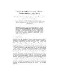
Sensor Meas. range Contact Abs/Inc Precision (µm) LVDT Small No Abs 250(*) Potentiometric Medium Yes Abs 400 Magnetostrictive Large No Abs 200 Optical encoder Large No Inc 5 Laser interferometer Very large No Inc 0.1 Table 1: Characteristics of typical commercial linear position sensors: measurement range, contact between the cursor and the displacement axis, absolute/incremental nature and precision. The precision corresponds to a measuring range of 1000 mm, except for the LVDT(*), where it is 100 mm. WAVEGUIDE RECEIVER CURSOR MAGNETS u PULSE GENERATOR u DAMPER Figure 1: Conventional MS linear position sensor. 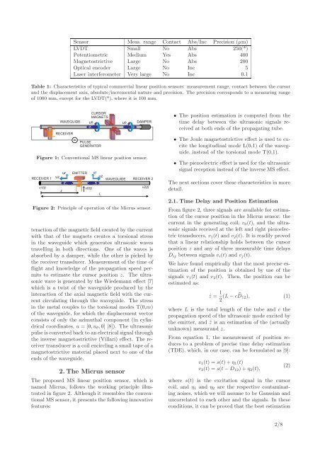ur EMITTER ur RECEIVER 1 uz uz WAVEGUIDE RECEIVER 2 v1(t) z v0(t) L v2(t) Figure 2: Principle of operation of the Micrus sensor. teraction of the magnetic field created by the current with that of the magnets creates a torsional stress in the waveguide which generates ultrasonic waves travelling in both directions. One of the waves is absorbed by a damper, while the other is picked by the receiver transducer. Measurement of the time of flight and knowledge of the propagation speed permits to estimate the cursor position z. The ultrasonic wave is generated by the Wiedemann effect [7] which is a twist of the waveguide produced by the interaction of the axial magnetic field with the current circulating through the waveguide. The stress in the metal couples to the torsional modes T(0,m) of the waveguide, for which the displacement vector consists of only the azimuthal component (in cylindrical coordinates, u = [0,u θ ,0] [8]). The ultrasonic pulse is converted back to an electrical signal through the inverse magnetostrictive (Villari) effect. The receiver transducer is a coil encircling a small tape of a magnetostrictive material placed next to one of the ends of the waveguide. 2. The Micrus sensor The proposed MS linear position sensor, which is named Micrus, follows the working principle illustrated in figure 2. Although it resembles the conventional MS sensor, it presents the following innovative features: • The position estimation is computed from the time delay between the ultrasonic signals received at both ends of the propagating tube. • The Joule magnetostrictive effect is used to excite the longitudinal mode L(0,1) of the waveguide, instead of the torsional mode T(0,1). • The piezoelectric effect is used for the ultrasonic signal reception instead of the inverse MS effect. The next sections cover these characteristics in more detail. 2.1. Time Delay and Position Estimation From figure 2, three signals are available for estimation of the cursor position in the Micrus sensor: the current in the generating coil, v 0 (t), and the ultrasonic signals received at the left and right piezoelectric transducers, v 1 (t) and v 2 (t). It is readily proved that a linear relationship holds between the cursor position z and any of three measurable time delays D ij between signals v i (t) and v j (t). We have found empirically that the most precise estimation of the position is obtained by use of the signals v 1 (t) and v 2 (t). Then, the position can be estimated as: ẑ = 1 2 (L − c ̂D 12 ), (1) where L is the total length of the tube and c the propagation speed of the ultrasonic mode excited by the emitter, and ẑ is an estimation of the (actually unknown) measurand z. From equation 1, the measurement of position reduces to a problem of precise time delay estimation (TDE), which, in our case, can be formulated as [9]: v 1 (t) = s(t) + η 1 (t) v 2 (t) = s(t − D 12 ) + η 2 (t), (2) where s(t) is the excitation signal in the cursor coil, and η 1 and η 2 are the respective contaminating noises, which we will assume to be Gaussian and uncorrelated to each other and the signals. In these conditions, it can be proved that the best estimation 2/8
of the time delay ̂D 12 is yielded by the value that maximizes the correlation of signals: ∫ ̂D 12 = max arg{ ̂R 12 (τ) = v 1 (t)v 2 (t − τ)dt}. (3) The Cramér-Rao lower bound (CRLB) [10] sets a limit on the maximum accuracy which can be achieved in the estimation of the time delay from the set of equations 2. The standard deviation σ D of the estimation of the delay ̂D is: σD 2 1 ≥ 16π 2 BTf0 2 (4) SNR, a result which is applicable in the case of narrowband signals with central frequency f 0 , and spectra contained in the interval |f| ∈ [f 0 −B,f 0 +B], where the bandwidth B is small with respect to f 0 . Likewise, the (linear) SNR must be high enough for unambiguous determination of the peak of the correlation R 12 (τ) [11]. The observation time, T, is, in practice, equal to the duration of the signal s(t). Another important nuance for the TDE process is that we will actually work with sampled versions v 1 [n] = v 1 (nt s ) and v 2 [n] = v 2 (nt s ) of the signals in equation 2 (t s is the sampling time). If we limit the precision in the estimation of the correlation peak to one sampling interval, the error committed can be as high as ±t s /2. For example, for a sampling frequency of f s = 2 MHz, and taking c ≃ 5 µm/ns in equation 1, the position error is bounded by σ z = 600 µm, which is clearly too high for a MS sensor. One method to estimate the time delay D 12 with subsample precision consists in fitting an analytical curve to the three samples closest to the discrete maximum [12] (note that this requires a minimum sampling frequency f s > 6f 0 in order to have at least three points in the positive semi-cycle of the correlation vector). The proper analytical curve to be fitted depends on the waveform s(t) used for excitation of the ultrasonic signals. In the Micrus sensor we have employed a sine train modulated by a Hanning window: [ 1 − cos( 2πt T ) ] [S H (t) − S H (t − T)] sinω 0 t, s(t) = 1 2 (5) where S H (t) is Heaviside’s step function, T = n cyc /f 0 is the total signal length, and n cyc is the number of cycles of the signal. This waveform does a good job in producing a finite duration signal with its energy contained in a small bandwidth. For the signal of equation 5, the correlation takes a cosine shape near the peak; thus, an improved estimation of the delay is obtained by fitting the following function: R[m] = acos(bm + c), (6) to the discrete maximum m max and its neighboring points. The improved time delay is estimated as: with: ̂D cos = (m max − c b )t s, (7) cos b = ̂R[m max − 1] + ̂R[m max + 1] 2 ̂R[m max ] tan c = ̂R[m max − 1] − ̂R[m max + 1] 2 ̂R[m . max ]sin b 2.2. Selection of the propagating mode (8) A waveguide with cylindrical symmetry can support three families of modes: torsional (denoted T(0,m)), longitudinal (L(0,m)) and flexural (F(n,m)) [8]. As the index n stands for the order of symmetry around the z axis, the torsional and longitudinal modes are axisymmetric (n = 0), while the flexural modes are asymmetric. The index m is used to order the propagating modes which can coexist in a family for a given operating frequency. In general, in any application which involves ultrasonic waves in solids, exploitation of a single propagating mode is recommended [13]. Ultrasonic signals travelling in a waveguide are subject to the phenomenon of dispersion, which is the variation of the phase and group speeds of the propagating waves with frequency. The theoretical dispersion curves in the low frequency range for the torsional, longitudinal and first two families of flexural modes are computed with the PCDISP software described in reference [14] and shown in figure 3. It can be acknowledged from the figure that the mode T(0,1) has the unique feature of being free from dispersive effects. This is one reason that leads to its use in the commercial MS sensors that we saw in section 1. In the Micrus sensor, however, we are interested in exploring the possibilities of using the faster propagating first longitudinal mode L(0,1) for position measurement. With a new design of the emitter it is possible to obtain high transduction efficiency in the generation and reception processes, achieving the SNR required by equation 4 for accurate estimation of the time delay. For the L(0,1) mode, the displacement vector has two nonzero entries u = [u r ,0,u z ]; however, at low frequencies, the radial component is much smaller than the axial one, u r ≪ u z . One consequence of choosing the mode L(0,1) for operation of our sensor is that we need to quantify the effects of dispersion, unlike the case of the torsional mode. Because the frequency components of the signal travel at different phase speeds, the signal is distorted as it propagates along the waveguide. When those signals are used in the time delay and position 3/8
Page 1: A High Accuracy Magnetostrictive Li
Page 5 and 6: STEEL TUBE PIEZOELECTRIC CERAMIC ME
Page 7 and 8: OPTICAL ENCODER RECEIVER 1 DRIVER E

Download PDF - Centro de Automática y Robótica

You also want an ePaper? Increase the reach of your titles

Delete template?

Save as template?