A High Accuracy Magnetostrictive Linear Position Sensor

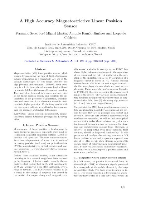
A High Accuracy Magnetostrictive Linear PositionSensorFernando Seco, José Miguel Martín, Antonio Ramón Jiménez and LeopoldoCalderónInstituto de Automática Industrial, CSIC.Ctra. de Campo Real, km 0,200, 28500 Arganda del Rey, Madrid, SpainCorresponding e-mail: fseco@iai.csic.esWebpage: http://www.iai.csic.es/users/lopsiPublished in Sensors & Actuators A, vol. 123–4, pp. 216-223 (sep. 2005)AbstractMagnetostrictive (MS) linear position sensors, whichoperate by measuring the time of flight of ultrasonicsignals propagating in a waveguide, are one of thepossible technologies for long range, absolute andhigh precision measurement. However, their accuracyis still far from the micrometer level achievedby standard differential sensors like optical encoders.This paper describes work in progress in a novel kindof MS linear position sensor, and considers the optimizationof the processes of generation, transmissionand reception of the ultrasonic waves in orderto obtain higher precision. Preliminary results withthe new sensor indicate a considerable improvementover the accuracy of standard MS sensors.Keywords: Linear position measurement, magnetostrictivesensors ultrasonic propagation in waveguides.1. Linear Position SensorsMeasurement of linear position is fundamental inmany industrial processes, especially when used forfeedback in computer numerical controls (CNC) formachine tool operation. The most common sensors,for a linear displacement of about 1 m, in order ofincreasing precision (and cost) are potentiometers,LVDTs, magnetostrictive, optical encoders and laserinterferometers [1]. Their characteristics are summarizedin table 1.Besides these standard sensors, other alternativetechnologies in a research stage have been reportedin the literature. A linear encoder based in the capacitiveeffect is described in [2], with non-linearityof 40 µm (accuracy of 3 µm after calibration) over arange of 150 mm. The PLCD sensor reported in [3]is based in the change of magnetic flux caused bythe motion of a magnet along a soft magnetic core;this sensor is similar in concept to an LVDT, butshows higher tolerance to changes in the separationof the cursor and the ruler. A similar idea, the variationof the inductance in a coil by saturation of amagnetic circuit is shown in [4]. Already existingsensors benefit also from the new magnetic materialslike amorphous ribbons which are used as coreelements. These materials provide superior linearityin LVDTs [5], therefore extending the measurementrange of the device. They are also used as transmittingelements in displacement sensors based in magnetostrictivedelay lines [6], obtaining high accuracy(< 10 µm) over short ranges (20 mm).Magnetostrictive (MS) linear position sensors constitutean interesting possibility as generic all-use sensorsbecause they are by principle non-contact andabsolute. These are very desirable characteristics formachine tool operation, as well as their non-opticalnature which makes them resistant to typical contaminantsof the machine tool environment like shavingsand metalworking coolant fluid. However, inorder to be competitive with linear encoders, theiraccuracy should be improved considerably. In thispaper we will analyze the existing commercial MSlinear position sensor and propose an improved versionof it. Also we will show different aspects of itsdesign, aimed at achieving high measurement precision.Finally we will report preliminary experimentalresults with a prototype of a position sensor andstate some conclusions.1.1. Magnetostrictive linear position sensorsIn a MS sensor, the position is estimated from thetime-of-flight (TOF) of ultrasonic signals generatedin a waveguide at the mobile element by the magnetostrictiveeffect. The basic setup is shown in figure1. The sensor consists in a ferromagnetic waveguide(usually a wire or a thin tube) that covers the1/9

Sensor Meas. range Contact Abs/Inc Precision (µm)LVDT Small No Abs 250(*)Potentiometric Medium Yes Abs 400Magnetostrictive Large No Abs 200Optical encoder Large No Inc 5Laser interferometer Very large No Inc 0.1Table 1: Characteristics of typical commercial linear position sensors: measurement range, contact between the cursorand the displacement axis, absolute/incremental nature and precision. The precision corresponds to a measuring rangeof 1000 mm, except for the LVDT(*), where it is 100 mm.WAVEGUIDERECEIVERCURSORMAGNETSuPULSEGENERATORuDAMPERFigure 1: Conventional MS linear position sensor.ur EMITTER urRECEIVER 1uzuzWAVEGUIDE RECEIVER 2v1(t)zv0(t)Lv2(t)Figure 2: Principle of operation of the Micrus sensor.measuring length, and a cursor formed by a set ofmagnets oriented perpendicularly to the tube, movingalong the waveguide. Periodically a pulse generatorsends an electric signal through the tube; the interactionof the magnetic field created by the currentwith that of the magnets creates a torsional stressin the waveguide which generates ultrasonic wavestravelling in both directions. One of the waves isabsorbed by a damper, while the other is picked bythe receiver transducer. Measurement of the time offlight and knowledge of the propagation speed permitsto estimate the cursor position z. The ultrasonicwave is generated by the Wiedemann effect [7]which is a twist of the waveguide produced by theinteraction of the axial magnetic field with the currentcirculating through the waveguide. The stressin the metal couples to the torsional modes T(0,m)of the waveguide, for which the displacement vectorconsists of only the azimuthal component (in cylindricalcoordinates, u = [0,u θ ,0] [8]). The ultrasonicpulse is converted back to an electrical signal throughthe inverse magnetostrictive (Villari) effect. The receivertransducer is a coil encircling a small tape of amagnetostrictive material placed next to one of theends of the waveguide.2. The Micrus sensorThe proposed MS linear position sensor, which isnamed Micrus, follows the working principle illustratedin figure 2. Although it resembles the conventionalMS sensor, it presents the following innovativefeatures:• The position estimation is computed from thetime delay between the ultrasonic signals receivedat both ends of the propagating tube.• The Joule magnetostrictive effect is used to excitethe longitudinal mode L(0,1) of the waveguide,instead of the torsional mode T(0,1).• The piezoelectric effect is used for the ultrasonicsignal reception instead of the inverse MS effect.The next sections cover these characteristics in moredetail.2.1. Time Delay and Position EstimationFrom figure 2, three signals are available for estimationof the cursor position in the Micrus sensor: thecurrent in the generating coil, v 0 (t), and the ultrasonicsignals received at the left and right piezoelectrictransducers, v 1 (t) and v 2 (t). It is readily provedthat a linear relationship holds between the cursorposition z and any of three measurable time delaysD ij between signals v i (t) and v j (t).We have found empirically that the most precise estimationof the position is obtained by use of thesignals v 1 (t) and v 2 (t). Then, the position can beestimated as:ẑ = 1 2 (L − c ̂D 12 ), (1)where L is the total length of the tube and c thepropagation speed of the ultrasonic mode excited bythe emitter, and ẑ is an estimation of the (actuallyunknown) measurand z.From equation 1, the measurement of position reducesto a problem of precise time delay estimation(TDE), which, in our case, can be formulated as [9]:v 1 (t) = s(t) + η 1 (t)v 2 (t) = s(t − D 12 ) + η 2 (t),(2)2/9

where s(t) is the excitation signal in the cursorcoil, and η 1 and η 2 are the respective contaminatingnoises, which we will assume to be Gaussian anduncorrelated to each other and the signals. In theseconditions, it can be proved that the best estimationof the time delay ̂D 12 is yielded by the value thatmaximizes the correlation of signals:∫̂D 12 = max arg{ ̂R 12 (τ) = v 1 (t)v 2 (t − τ)dt}. (3)The Cramér-Rao lower bound (CRLB) [10] setsa limit on the maximum accuracy which can beachieved in the estimation of the time delay fromthe set of equations 2. The standard deviation σ D ofthe estimation of the delay ̂D is:σD 2 1≥16π 2 BTf0 2 (4)SNR,a result which is applicable in the case of narrowbandsignals with central frequency f 0 , and spectra containedin the interval |f| ∈ [f 0 −B,f 0 +B], where thebandwidth B is small with respect to f 0 . Likewise,the (linear) SNR must be high enough for unambiguousdetermination of the peak of the correlationR 12 (τ) [11]. The observation time, T, is, in practice,equal to the duration of the signal s(t).Another important nuance for the TDE process isthat we will actually work with sampled versionsv 1 [n] = v 1 (nt s ) and v 2 [n] = v 2 (nt s ) of the signalsin equation 2 (t s is the sampling time). If welimit the precision in the estimation of the correlationpeak to one sampling interval, the error committedcan be as high as ±t s /2. For example, fora sampling frequency of f s = 2 MHz, and takingc ≃ 5 µm/ns in equation 1, the position error isbounded by σ z = 600 µm, which is clearly too highfor a MS sensor.One method to estimate the time delay D 12 withsubsample precision consists in fitting an analyticalcurve to the three samples closest to the discretemaximum [12] (note that this requires a minimumsampling frequency f s > 6f 0 in order to have at leastthree points in the positive semi-cycle of the correlationvector). The proper analytical curve to be fitteddepends on the waveform s(t) used for excitation ofthe ultrasonic signals. In the Micrus sensor we haveemployed a sine train modulated by a Hanning window:[1 − cos( 2πtT ) ][S H (t) − S H (t − T)] sinω 0 t,s(t) = 1 2(5)where S H (t) is Heaviside’s step function, T =n cyc /f 0 is the total signal length, and n cyc is thenumber of cycles of the signal. This waveform doesa good job in producing a finite duration signal withits energy contained in a small bandwidth.For the signal of equation 5, the correlation takes acosine shape near the peak; thus, an improved estimationof the delay is obtained by fitting the followingfunction:R[m] = acos(bm + c), (6)to the discrete maximum m max and its neighboringpoints. The improved time delay is estimated as:with:̂D cos = (m max − c b )t s, (7)cos b = ̂R[m max − 1] + ̂R[m max + 1]2 ̂R[m max ]tan c = ̂R[m max − 1] − ̂R[m max + 1]2 ̂R[m.max ]sin b2.2. Selection of the propagating mode(8)A waveguide with cylindrical symmetry can supportthree families of modes: torsional (denoted T(0,m)),longitudinal (L(0,m)) and flexural (F(n,m)) [8]. Asthe index n stands for the order of symmetry aroundthe z axis, the torsional and longitudinal modes areaxisymmetric (n = 0), while the flexural modes areasymmetric. The index m is used to order the propagatingmodes which can coexist in a family for agiven operating frequency. In general, in any applicationwhich involves ultrasonic waves in solids,exploitation of a single propagating mode is recommended[13].Ultrasonic signals travelling in a waveguide are subjectto the phenomenon of dispersion, which is thevariation of the phase and group speeds of the propagatingwaves with frequency. The theoretical dispersioncurves in the low frequency range for the torsional,longitudinal and first two families of flexuralmodes are computed with the PCDISP software describedin reference [14] and shown in figure 3.It can be acknowledged from the figure that the modeT(0,1) has the unique feature of being free from dispersiveeffects. This is one reason that leads to itsuse in the commercial MS sensors that we saw in section1. In the Micrus sensor, however, we are interestedin exploring the possibilities of using the fasterpropagating first longitudinal mode L(0,1) for positionmeasurement. With a new design of the emitterit is possible to obtain high transduction efficiency inthe generation and reception processes, achieving theSNR required by equation 4 for accurate estimationof the time delay. For the L(0,1) mode, the displacementvector has two nonzero entries u = [u r ,0,u z ];3/9

Phase speed (m/s)Group speed (m/s)80007000600050004000300020001000(a)F(1,1)F(2,1)L(0,1)T(0,1)F(1,2)L(0,2)00 50 100 150 200 250 300Frequency (kHz)600050004000300020001000(b)F(1,1)F(2,1)T(0,1)L(0,1)F(1,2)L(0,2)00 50 100 150 200 250 300Frequency (kHz)Figure 3: (a) Phase and (b) group speed curves for thetorsional T(0,m), longitudinal L(0,m) and first two flexuralmodes, F(1,m) and F(2,m), existing in the frequencyrange 0-300 kHz, computed with PCDISP. The tube datais given in section 3.1.however, at low frequencies, the radial component ismuch smaller than the axial one, u r ≪ u z .One consequence of choosing the mode L(0,1) for operationof our sensor is that we need to quantify theeffects of dispersion, unlike the case of the torsionalmode. Because the frequency components of the signaltravel at different phase speeds, the signal is distortedas it propagates along the waveguide. Whenthose signals are used in the time delay and positionestimation processes, the result is a systematic (i.e.,position dependent) error in the measurement.Several precautions can be taken to minimize the effectsof dispersion. The width of the flat region ofthe L(0,1) curve in figure 3 depends inversely on thethickness of the tube, so the thinnest available tubeshould be used. The excitation signal s(t) shouldhave a narrow spectral content, and the central frequencyf 0 lie in a point where the dispersion curveis relatively flat (dc ph /dω ≃ 0).Where dispersion is unavoidable, theoretical or empiricalknowledge of the wavenumber-frequency relationship,ξ(ω), can be used to compensate the distortionsuffered by the signal during the propagation inthe waveguide. For example, Gorham and Wu [15]were able to restore the original shape of stress pulsescaused by impact of steel spheres in pressure bars.Wilcox [16] has developed an optimized algorithmbased on use of the FFT which could be employedfor real time correction of dispersive effects.To check if these methods are really needed, we performedsimulations of the propagation of signals inthe tube employed in the Micrus system, and theposition estimation method of equation 1, for a totaldisplacement range of 1 m. Using the softwarePCDISP and the method described in [17], we studiedthe influence of two design parameters of thewaveform s(t) of equation 5: the central frequencyf 0 and the number of cycles n cyc , on the positionestimation. The results are shown in figure 4 (thephysical data for the transmitting tube is given insection 3.1. As expected, the position error increaseswith frequency, as the dispersion curve ofmode L(0,1) in figure 3 gets steeper and closer tothe cutting frequency of mode L(0,2). The positionerror decreases with growing signal length (narrowerspectral content), becoming lower than 1 µmfor n cyc > 4 cycles. This is very convenient, becauseit allows to use relatively short (temporal orspatial) excitation signals, and obtain a longer measuringrange for a given tube size.As a conclusion of the simulation process, active correctionof the dispersion effects is not needed for operatingfrequencies below 100 kHz, unless the errordue to other sources is inferior to 2 µm.2.3. Magnetostrictive EmitterThe emitter transducer of the Micrus system is designedto produce maximum coupling to the chosenultrasonic mode (longitudinal L(0,1)). To this endthe Joule magnetostrictive effect (in which the staticand dynamic fields are arranged in the axial direction[7]) is used instead of the Wiedemann effect.The emitter transducer, shown in figure 5, consistsmainly of two elements. A set of four Alcomax IIImagnets provide a bias field which brings the partof the tube under the cursor to a known state in themagnetization curve, reducing hysteretic effects andincreasing measurement repeatability. In the centralregion, an excitation coil (10 mm long, consisting of60 turns of copper wire), creates the dynamic signalresponsible of the MS generation. The total field isthen given by H(z) = H 0 + H 1 expj2πf 0 t, with H 1being about 10 times smaller in magnitude than H 0 ,in order to reduce harmonics created by the nonlineargeneration of ultrasound.4/9

STEEL TUBEPIEZOELECTRICCERAMIC2.521.51(a) Excitation frequency f 0METALLICPLATEV PIEZOError (µm)0.50−0.5−1−1.5−2f 0=40 kHzf 0=60 kHzf 0=80 kHz−2.50 100 200 300 400 500 600 700 800 900 1000Position (mm)Error (µm)3210−1−2(b) Number of cycles2 cycles4 cycles6 cycles−30 100 200 300 400 500 600 700 800 900 1000Position (mm)Figure 4: Simulation of the influence of (a) the centralfrequency f 0 (with n cyc = 6); and (b) the number ofcycles n cyc (with f 0 = 60 kHz) of the excitation signals(t) on the systematic error in the position estimation.Figure 5: Magnetostrictive emitter of the Micrus sensor.ALUMINUMADAPTERFigure 6: Arrangement of the piezoelectric receivertransducer at the end of the propagating tube.Operation with the prototype showed that the positionestimation process suffered from measurementhysteresis, caused in turn by the magnetic hysteresisof the metal of the transmitting element. A methodwas devised to compensate this problem, by focusingthe dynamic magnetic field and choosing a convenientmaterial (duplex stainless steel) for the propagatingtube; more details of this procedure can befound in reference [18].2.4. Piezoelectric receiverWe decided to use the piezoelectric effect instead ofthe inverse (Villari) magnetostrictive effect in orderto enhance the sensitivity of the receivers and increasethe SNR for the TDE process (as required byequation 4). Because there are no mobility requirementson the receiver transducers, they are simplystuck at the ends of the tube.Excellent sensitivity to low frequency (f 0 < 100 kHz)ultrasonic waves in the tube was obtained with MurataMA40B8R piezoceramic disks. Each transducerwas attached to the end of the tube with an aluminumadapter (see figure 6), which served to enhancethe reproducibility of the measurements andobtain a higher correlation level between signals v 1 (t)and v 2 (t).2.5. Selection of excitation frequency (f 0 )The experimental gain of the whole transducer system(comprising the processes of magnetostrictivegeneration, transmission in the waveguide and piezoelectricreception) is shown in figure 7. The responseof the system is contained mainly in the 20-140 kHzrange, achieving the maximum gain at 80 kHz, andwith a second peak at a very low frequency (25 kHz).This second maximum corresponds to a resonance ofthe adapter piece.Besides high gain, it is also desirable to obtain highcorrelation between the emitted and received signals,for optimal results of the correlation algorithm. Anexcitation frequency close to the maximum amplitudepoint (80 kHz) causes signal ringing and deterioratesthe correlation value. Experimental waveforms5/9

Gain (dB)3025201510500 50 100 150 200Frequency (kHz)Figure 7: Experimental frequency response of themagnetostrictive-piezoelectric transduction process inthe Micrus system.6420−2−4f =60 kHz0R=0.969f =70 kHz0R=0.923f =80 kHz0R=0.959f =90 kHz0R=0.881f =100 kHz0R=0.901for different values of the frequency f 0 along with thenormalized correlation, are shown in figure 8, wherethe excitation waveform is given by equation 5 withn cyc = 8.With help of the data in this figure we finally selectedthe excitation frequency for Micrus as f 0 = 60 kHz.Lower frequencies, which empirically provide evenhigher correlation values, were avoided to keep thesignal length down.3. Empirical resultsIn this part we will describe the physical prototype inwhich we implemented the techniques of the last sectionand provide some experimental measurementsobtained with the sensor.3.1. Micrus prototypeThe Micrus linear position sensor is shown in figure 9.The excitation signal (equation 5) is created in thecentral PC and transmitted via the GPIB bus to anarbitrary waveform generator (Agilent 33120A), filteredby an RC filter to smooth out the quantizationsteps of the 8-bit signal generator, amplified by adriver (ENI model 240L, with a gain of 50 dB) andput into the emitter coil. The current through thiscoil (signal v 0 (t) in figure 2) is measured with a 0.1 Ωsensing resistance in series.The transmitting waveguide is a stainless duplexsteel tube (Sandvik SAF2304), with outer diameter8 mm and thickness of 1 mm, and a total length of1600 mm. The measurable range is 1000 mm, becausea guard distance at both sides must be leftto avoid interference of the emitted signals and theechoes from the extremes of the tube. This is knownto be a limiting factor of the accuracy obtainablewith magnetostrictive sensors [19]. The speed of−650 100 150 200 250 300 350Time (µs)Figure 8: Emitted (light line) and received (dark line)signals for different excitation frequencies f 0 (signals havebeen normalized to unit amplitude), and values of theircross correlation.sound of the L(0,1) mode at 60 kHz is very closeto the bar velocity, c 0 = 5060 m/s. The tube is fixedto an optical bench (Newport X95-2), and held bysilicon supports to avoid mechanical loading of thepropagating ultrasonic waves. A commercial opticalencoder (Fagor Automation model CX 1545, withrange of 1.5 m and rated accuracy ±5 µm) is installedon the same frame for calibration and measurementof error purposes. The measurement is displayedin a digital readout and transmitted to thecontrol PC through the serial port.After reception of the propagating ultrasonic signalsby the piezoceramics, they are amplified by instrumentationamplifiers, and isolated and decoupledwith pulse transformers to achieve a high commonmode rejection ratio. The three signals v 0 (t), v 1 (t)and v 2 (t) are simultaneously digitized with an acquisitioncard (Adlink PCI-9812), with a sampling frequencyranging between 1 and 5 MHz. The PC processesthe acquired signals with an IIR Butterworthlowpass digital filter, with the cutoff frequency set at2f 0 , in order to reject the out of band and quantizationnoise, and improve the SNR. The PC also runsthe time delay and position estimation algorithmsand provides a graphical interface and data analysiscapabilities.6/9

OPTICAL ENCODERRECEIVER 1DRIVEREMITTERI IIIIIIIIIIIII IIIIIIIIIICURSORWAVEGUIDESIGNALGENERATORRECEIVER 2V1(t) V0(t) SYNCHRONIZATIONV2(t)GPIBBUSACQUISITIONCARDSERIALPORTDIGITAL READOUTX 23.475Y 0.110Z -102.240Figure 9: Block diagram of the prototype of the Micrus sensor.The experimental prototype of the Micrus sensor justdescribed was created with flexibility in mind, in orderto permit modifications during its development.For this reason, standard laboratory equipment anda common PC have been used in its design. In a preindustrialversion a suitable DSP would substitutethe PC, the function generator and the acquisitioncard used in the creation, reception and processing ofthe ultrasonic signals; with custom electronic driversand amplifiers being incorporated into the sensor.The final cost of the sensor could be considerablycheaper than that of a quality optical encoder, sinceno expensive element like a glass substrate with thegrating is needed.3.2. Position measurementA first experiment was performed to obtain empiricaldata of the variation of the time delay with thesampling frequency (f s ), recorded at a static positionof the cursor close to the middle of the measuringrange. Results for three sampling frequenciesare shown in table 2. Oversampling the signals withf s ≫ f 0 is advantageous because it is equivalent inpractice to increasing the SNR, and therefore, reducingthe standard deviation of the TDE process,according to equation 4. Setting the sampling frequencyas f s = 2 MHz, we obtain a dispersion in themeasurements of 3.4 ns, which means that the precisionof the sensor can be taken as 8 µm. However,the position repeatability, i.e., the difference of themeasured values when the same reference position isreached several times, is higher, typically equal to10 µm. This is a value twice as large of that of theoptical encoder used for reference.The dynamic behavior of the sensor was obtained bySampling frequency,Time delay Position er-f s error, σ D ror, σ z (µm)(MHz) (ns)1 14.4 362 3.4 8.55 1.4 3.5Table 2: Standard deviation of the estimation of timedelay and position in the Micrus system, with respect tothe sampling frequency.moving the cursor in several cycles that covered thewhole displacement range (1000 mm), recording theposition estimation of Micrus and the measurementof the reference optical encoder. The difference betweenthem, ẑ[Micrus] − ẑ[encoder] is graphed as anerror curve in figure 10. The nonlinearity is boundedby ±30 µm in the whole range of the sensor. Whilethis is still too high for machine tool operation, theprecision is about 6 times better than that of conventionalmagnetostrictive linear position sensors (describedin section 1.1). The error pattern is quiterepetitive, and characteristic of the tube used; webelieve that it ultimately corresponds to the mechanicaland magnetic inhomogeneities of the tube thatserves as propagating medium for the ultrasonic signal.One important aspect of the operation of the Micrussensor which needs to be commented is the influenceof temperature on the position measurement. In opticalencoders, the main effect is the expansion of thesubstrate material, which for glass is typically about10 −5 o C −1 . The thermal behavior of the substrate iswell known, to the point that some encoder manufacturersoffer products with expansion characteristics7/9

Error (µm)403020100−10−20−30−400 200 400 600 800 1000Position (mm)Figure 10: Typical error curve of the Micrus sensor,computed as the difference between the position estimationand the commercial optical encoder output. Threecycles over the whole measuring range are shown.which match those of the machine tool in which theywill be used. In magnetostrictive sensors, the mostinfluential factor is rather the change of the propagationspeed of the ultrasonic wave (in the order of10 −4 o C −1 for steel). In the laboratory experimentof figure 10, the temperature was kept constant at25 ± 0.25 o C. For operation in realistic machine-toolenvironments, some method of active temperaturecompensation should be included (for example, integratinga temperature sensor in Micrus).4. ConclusionsIn this paper we have proposed a novel design of amagnetostrictive (MS) linear position sensor, whichdiffers in several aspects from the existing sensors,and is intended to provide higher accuracy. Themodifications include the measurement principle, thepropagating mode selected and the receiver transducer.The results with a prototype MS linear position sensor(Micrus) built according to those principles haveshown an accuracy of ±30 µm over a 1 m range, significantlyimproving the performance of existing sensors.We believe that the precision is ultimately limitedby the mechanical and magnetic homogeneity of thetube which serves as the propagating element of theultrasonic signals. The regularity of the obtainederror pattern suggests that further improvements ofthe position sensor are possible and that the precisionof MS linear position sensors may come closerto that of optical encoders.References[1] J. G. Webster (Ed.), The Measurement, Instrumentationand Sensors Handbook, The ElectricalEngineering Handbook Series, CRC Press,Springer and IEEE Press, 1999.[2] M. H. W. Bonse, F. Zhu, H. F. van Beek, Along-range capacitive displacement sensor havingmicrometre resolution, Meas. Sci. Technol.4 (8) (1993) 801–807.[3] O. Erb, G. Hinz, N. Preusse, PLCD, a novelmagnetic displacement sensor, Sensors and ActuatorsA 25-27 (1991) 277–282.[4] B. Legrand, Y. Dordet, J.-Y. Voyant, J.-P. Yonnet,Contactless position sensor using magneticsaturation, Sensors and Actuators A 106 (1-3)(2003) 149–154.[5] T. Meydan, G. W. Healey, Linear variable differentialtransformer (LVDT): linear displacementtransducer utilizing ferromagnetic amorphousmetallic glass ribbons, Sensors and ActuatorsA 32 (1992) 582–587.[6] V. Karagiannis, C. Manassis, D. Bargiotas, Positionsensors based on the delay line principle,Sensors and Actuators A 106 (1-3) (2003) 183–186.[7] E. du Trémolet de Lacheisserie, Magnetostriction:Theory and applications of magnetoelasticity,CRC Press, 1993.[8] D. C. Gazis, Three-dimensional investigationof the propagation of waves in hollow circularcylinders. I. Analytical foundation. II. Numericalresults., J. Acoust. Soc. Am. 31 (5) (1959)568–578.[9] G. C. Carter, Coherence and time delay estimation,Proceedings of the IEEE 75 (2) (1987)236–255.[10] J. Minkoff, Signals, Noise and Active Sensors,1st Edition, Wiley Interscience, 1992.[11] A. Zeira, P. M. Schultheiss, Realizable lowerbounds for time delay estimation: Part 2 -Threshold phenomena, IEEE Trans. on SignalProcessing 42 (5) (1994) 1001–1007.[12] I. Céspedes, Y. Huang, J. Ophir, S. Spratt,Methods for estimation of subsample time delaysof digitized echo signals, Ultrasonic Imaging17 (2) (1995) 142–171.[13] J. L. Rose, Ultrasonic Waves in Solid Media, 1stEdition, Cambridge University Press, 1999.[14] F. Seco, J. M. Martín, A. R. Jiménez, J. L. Pons,L. Calderón, R. Ceres, PCDISP: a tool for thesimulation of wave propagation in cylindricalwaveguides, in: 9th International Congress onSound and Vibration, Orlando, Florida, USA,July 8-11, 2002, p. 23.[15] D. A. Gorham, X. J. Wu, An empirical methodfor correcting dispersion in pressure bar mea-8/9

surements of impact stress, Meas. Sci. Technol.7 (9) (1996) 1227–1232.[16] P. D. Wilcox, A rapid signal processing techniqueto remove the effect of dispersion fromguided wave signals, IEEE Transactions on Ultrasonics,Ferroelectrics and Frequency Control50 (4) (2003) 419–427.[17] J. F. Doyle, Wave Propagation in Structures,2nd Edition, Springer, 1997.[18] F. Seco, J. M. Martín, J. L. Pons, A. R. Jiménez,Hysteresis compensation in a magnetostrictivelinear position sensor, Sensors and Actuators A110 (1-3) (2004) 247–253.[19] A. Affanni, A. Guerra, L. Dallagiovanna,G. Chiorboli, Design and characterization ofmagnetostrictive linear displacement sensors, in:Instrumentation and Measurement TechnologyConference, IMTC 2004, Como, Italy, May 18-20, 2004, pp. 206–209.9/9