Download PDF - Centro de Automática y Robótica

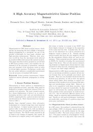
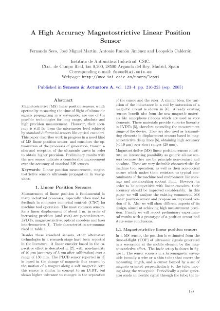
A High Accuracy Magnetostrictive Linear Position
Sensor
Fernando Seco, José Miguel Martín, Antonio Ramón Jiménez and Leopoldo Calderón
Instituto de Automática Industrial, CSIC.
Ctra. de Campo Real, km 0,200, 28500 Arganda del Rey, Madrid, Spain
Corresponding e-mail: fseco@iai.csic.es
Webpage: http://www.iai.csic.es/users/lopsi
Published in Sensors & Actuators A, vol. 123–4, pp. 216-223 (sep. 2005)
Abstract
Magnetostrictive (MS) linear position sensors, which
operate by measuring the time of flight of ultrasonic
signals propagating in a waveguide, are one of the
possible technologies for long range, absolute and
high precision measurement. However, their accuracy
is still far from the micrometer level achieved
by standard differential sensors like optical encoders.
This paper describes work in progress in a novel kind
of MS linear position sensor, and considers the optimization
of the processes of generation, transmission
and reception of the ultrasonic waves in order
to obtain higher precision. Preliminary results with
the new sensor indicate a considerable improvement
over the accuracy of standard MS sensors.
Keywords: Linear position measurement, magnetostrictive
sensors ultrasonic propagation in waveguides.
1. Linear Position Sensors
Measurement of linear position is fundamental in
many industrial processes, especially when used for
feedback in computer numerical controls (CNC) for
machine tool operation. The most common sensors,
for a linear displacement of about 1 m, in order of
increasing precision (and cost) are potentiometers,
LVDTs, magnetostrictive, optical encoders and laser
interferometers [1]. Their characteristics are summarized
in table 1.
Besides these standard sensors, other alternative
technologies in a research stage have been reported
in the literature. A linear encoder based in the capacitive
effect is described in [2], with non-linearity
of 40 µm (accuracy of 3 µm after calibration) over a
range of 150 mm. The PLCD sensor reported in [3]
is based in the change of magnetic flux caused by
the motion of a magnet along a soft magnetic core;
this sensor is similar in concept to an LVDT, but
shows higher tolerance to changes in the separation
of the cursor and the ruler. A similar idea, the variation
of the inductance in a coil by saturation of a
magnetic circuit is shown in [4]. Already existing
sensors benefit also from the new magnetic materials
like amorphous ribbons which are used as core
elements. These materials provide superior linearity
in LVDTs [5], therefore extending the measurement
range of the device. They are also used as transmitting
elements in displacement sensors based in magnetostrictive
delay lines [6], obtaining high accuracy
(< 10 µm) over short ranges (20 mm).
Magnetostrictive (MS) linear position sensors constitute
an interesting possibility as generic all-use sensors
because they are by principle non-contact and
absolute. These are very desirable characteristics for
machine tool operation, as well as their non-optical
nature which makes them resistant to typical contaminants
of the machine tool environment like shavings
and metalworking coolant fluid. However, in
order to be competitive with linear encoders, their
accuracy should be improved considerably. In this
paper we will analyze the existing commercial MS
linear position sensor and propose an improved version
of it. Also we will show different aspects of its
design, aimed at achieving high measurement precision.
Finally we will report preliminary experimental
results with a prototype of a position sensor and
state some conclusions.
1.1. Magnetostrictive linear position sensors
In a MS sensor, the position is estimated from the
time-of-flight (TOF) of ultrasonic signals generated
in a waveguide at the mobile element by the magnetostrictive
effect. The basic setup is shown in figure
1. The sensor consists in a ferromagnetic waveguide
(usually a wire or a thin tube) that covers the
measuring length, and a cursor formed by a set of
magnets oriented perpendicularly to the tube, moving
along the waveguide. Periodically a pulse generator
sends an electric signal through the tube; the in-
1/8

Sensor Meas. range Contact Abs/Inc Precision (µm)
LVDT Small No Abs 250(*)
Potentiometric Medium Yes Abs 400
Magnetostrictive Large No Abs 200
Optical encoder Large No Inc 5
Laser interferometer Very large No Inc 0.1
Table 1: Characteristics of typical commercial linear position sensors: measurement range, contact between the cursor
and the displacement axis, absolute/incremental nature and precision. The precision corresponds to a measuring range
of 1000 mm, except for the LVDT(*), where it is 100 mm.
WAVEGUIDE
RECEIVER
CURSOR
MAGNETS
u
PULSE
GENERATOR
u
DAMPER
Figure 1: Conventional MS linear position sensor.
ur EMITTER ur
RECEIVER 1
uz
uz
WAVEGUIDE RECEIVER 2
v1(t)
z
v0(t)
L
v2(t)
Figure 2: Principle of operation of the Micrus sensor.
teraction of the magnetic field created by the current
with that of the magnets creates a torsional stress
in the waveguide which generates ultrasonic waves
travelling in both directions. One of the waves is
absorbed by a damper, while the other is picked by
the receiver transducer. Measurement of the time of
flight and knowledge of the propagation speed permits
to estimate the cursor position z. The ultrasonic
wave is generated by the Wiedemann effect [7]
which is a twist of the waveguide produced by the
interaction of the axial magnetic field with the current
circulating through the waveguide. The stress
in the metal couples to the torsional modes T(0,m)
of the waveguide, for which the displacement vector
consists of only the azimuthal component (in cylindrical
coordinates, u = [0,u θ ,0] [8]). The ultrasonic
pulse is converted back to an electrical signal through
the inverse magnetostrictive (Villari) effect. The receiver
transducer is a coil encircling a small tape of a
magnetostrictive material placed next to one of the
ends of the waveguide.
2. The Micrus sensor
The proposed MS linear position sensor, which is
named Micrus, follows the working principle illustrated
in figure 2. Although it resembles the conventional
MS sensor, it presents the following innovative
features:
• The position estimation is computed from the
time delay between the ultrasonic signals received
at both ends of the propagating tube.
• The Joule magnetostrictive effect is used to excite
the longitudinal mode L(0,1) of the waveguide,
instead of the torsional mode T(0,1).
• The piezoelectric effect is used for the ultrasonic
signal reception instead of the inverse MS effect.
The next sections cover these characteristics in more
detail.
2.1. Time Delay and Position Estimation
From figure 2, three signals are available for estimation
of the cursor position in the Micrus sensor: the
current in the generating coil, v 0 (t), and the ultrasonic
signals received at the left and right piezoelectric
transducers, v 1 (t) and v 2 (t). It is readily proved
that a linear relationship holds between the cursor
position z and any of three measurable time delays
D ij between signals v i (t) and v j (t).
We have found empirically that the most precise estimation
of the position is obtained by use of the
signals v 1 (t) and v 2 (t). Then, the position can be
estimated as:
ẑ = 1 2 (L − c ̂D 12 ), (1)
where L is the total length of the tube and c the
propagation speed of the ultrasonic mode excited by
the emitter, and ẑ is an estimation of the (actually
unknown) measurand z.
From equation 1, the measurement of position reduces
to a problem of precise time delay estimation
(TDE), which, in our case, can be formulated as [9]:
v 1 (t) = s(t) + η 1 (t)
v 2 (t) = s(t − D 12 ) + η 2 (t),
(2)
where s(t) is the excitation signal in the cursor
coil, and η 1 and η 2 are the respective contaminating
noises, which we will assume to be Gaussian and
uncorrelated to each other and the signals. In these
conditions, it can be proved that the best estimation
2/8

of the time delay ̂D 12 is yielded by the value that
maximizes the correlation of signals:
∫
̂D 12 = max arg{ ̂R 12 (τ) = v 1 (t)v 2 (t − τ)dt}. (3)
The Cramér-Rao lower bound (CRLB) [10] sets
a limit on the maximum accuracy which can be
achieved in the estimation of the time delay from
the set of equations 2. The standard deviation σ D of
the estimation of the delay ̂D is:
σD 2 1
≥
16π 2 BTf0 2 (4)
SNR,
a result which is applicable in the case of narrowband
signals with central frequency f 0 , and spectra contained
in the interval |f| ∈ [f 0 −B,f 0 +B], where the
bandwidth B is small with respect to f 0 . Likewise,
the (linear) SNR must be high enough for unambiguous
determination of the peak of the correlation
R 12 (τ) [11]. The observation time, T, is, in practice,
equal to the duration of the signal s(t).
Another important nuance for the TDE process is
that we will actually work with sampled versions
v 1 [n] = v 1 (nt s ) and v 2 [n] = v 2 (nt s ) of the signals
in equation 2 (t s is the sampling time). If we
limit the precision in the estimation of the correlation
peak to one sampling interval, the error committed
can be as high as ±t s /2. For example, for
a sampling frequency of f s = 2 MHz, and taking
c ≃ 5 µm/ns in equation 1, the position error is
bounded by σ z = 600 µm, which is clearly too high
for a MS sensor.
One method to estimate the time delay D 12 with
subsample precision consists in fitting an analytical
curve to the three samples closest to the discrete
maximum [12] (note that this requires a minimum
sampling frequency f s > 6f 0 in order to have at least
three points in the positive semi-cycle of the correlation
vector). The proper analytical curve to be fitted
depends on the waveform s(t) used for excitation of
the ultrasonic signals. In the Micrus sensor we have
employed a sine train modulated by a Hanning window:
[
1 − cos( 2πt
T ) ]
[S H (t) − S H (t − T)] sinω 0 t,
s(t) = 1 2
(5)
where S H (t) is Heaviside’s step function, T =
n cyc /f 0 is the total signal length, and n cyc is the
number of cycles of the signal. This waveform does
a good job in producing a finite duration signal with
its energy contained in a small bandwidth.
For the signal of equation 5, the correlation takes a
cosine shape near the peak; thus, an improved estimation
of the delay is obtained by fitting the following
function:
R[m] = acos(bm + c), (6)
to the discrete maximum m max and its neighboring
points. The improved time delay is estimated as:
with:
̂D cos = (m max − c b )t s, (7)
cos b = ̂R[m max − 1] + ̂R[m max + 1]
2 ̂R[m max ]
tan c = ̂R[m max − 1] − ̂R[m max + 1]
2 ̂R[m
.
max ]sin b
2.2. Selection of the propagating mode
(8)
A waveguide with cylindrical symmetry can support
three families of modes: torsional (denoted T(0,m)),
longitudinal (L(0,m)) and flexural (F(n,m)) [8]. As
the index n stands for the order of symmetry around
the z axis, the torsional and longitudinal modes are
axisymmetric (n = 0), while the flexural modes are
asymmetric. The index m is used to order the propagating
modes which can coexist in a family for a
given operating frequency. In general, in any application
which involves ultrasonic waves in solids,
exploitation of a single propagating mode is recommended
[13].
Ultrasonic signals travelling in a waveguide are subject
to the phenomenon of dispersion, which is the
variation of the phase and group speeds of the propagating
waves with frequency. The theoretical dispersion
curves in the low frequency range for the torsional,
longitudinal and first two families of flexural
modes are computed with the PCDISP software described
in reference [14] and shown in figure 3.
It can be acknowledged from the figure that the mode
T(0,1) has the unique feature of being free from dispersive
effects. This is one reason that leads to its
use in the commercial MS sensors that we saw in section
1. In the Micrus sensor, however, we are interested
in exploring the possibilities of using the faster
propagating first longitudinal mode L(0,1) for position
measurement. With a new design of the emitter
it is possible to obtain high transduction efficiency in
the generation and reception processes, achieving the
SNR required by equation 4 for accurate estimation
of the time delay. For the L(0,1) mode, the displacement
vector has two nonzero entries u = [u r ,0,u z ];
however, at low frequencies, the radial component is
much smaller than the axial one, u r ≪ u z .
One consequence of choosing the mode L(0,1) for operation
of our sensor is that we need to quantify the
effects of dispersion, unlike the case of the torsional
mode. Because the frequency components of the signal
travel at different phase speeds, the signal is distorted
as it propagates along the waveguide. When
those signals are used in the time delay and position
3/8

Phase speed (m/s)
8000
7000
6000
5000
4000
3000
2000
(a)
F(1,1)
F(2,1)
L(0,1)
T(0,1)
F(1,2)
L(0,2)
Error (µm)
2.5
2
1.5
1
0.5
0
−0.5
−1
−1.5
(a) Excitation frequency f 0
f 0
=40 kHz
f 0
=60 kHz
1000
−2
f 0
=80 kHz
0
0 50 100 150 200 250 300
Frequency (kHz)
6000
5000
(b)
L(0,1)
−2.5
0 100 200 300 400 500 600 700 800 900 1000
Position (mm)
3
2
(b) Number of cycles
Group speed (m/s)
4000
3000
2000
F(1,1)
T(0,1)
F(1,2)
L(0,2)
Error (µm)
1
0
−1
1000
F(2,1)
−2
2 cycles
4 cycles
6 cycles
0
0 50 100 150 200 250 300
Frequency (kHz)
Figure 3: (a) Phase and (b) group speed curves for the
torsional T(0,m), longitudinal L(0,m) and first two flexural
modes, F(1,m) and F(2,m), existing in the frequency
range 0-300 kHz, computed with PCDISP. The tube data
is given in section 3.1.
−3
0 100 200 300 400 500 600 700 800 900 1000
Position (mm)
Figure 4: Simulation of the influence of (a) the central
frequency f 0 (with n cyc = 6); and (b) the number of
cycles n cyc (with f 0 = 60 kHz) of the excitation signal
s(t) on the systematic error in the position estimation.
estimation processes, the result is a systematic (i.e.,
position dependent) error in the measurement.
Several precautions can be taken to minimize the effects
of dispersion. The width of the flat region of
the L(0,1) curve in figure 3 depends inversely on the
thickness of the tube, so the thinnest available tube
should be used. The excitation signal s(t) should
have a narrow spectral content, and the central frequency
f 0 lie in a point where the dispersion curve
is relatively flat (dc ph /dω ≃ 0).
Where dispersion is unavoidable, theoretical or empirical
knowledge of the wavenumber-frequency relationship,
ξ(ω), can be used to compensate the distortion
suffered by the signal during the propagation in
the waveguide. For example, Gorham and Wu [15]
were able to restore the original shape of stress pulses
caused by impact of steel spheres in pressure bars.
Wilcox [16] has developed an optimized algorithm
based on use of the FFT which could be employed
for real time correction of dispersive effects.
To check if these methods are really needed, we performed
simulations of the propagation of signals in
the tube employed in the Micrus system, and the
position estimation method of equation 1, for a total
displacement range of 1 m. Using the software
PCDISP and the method described in [17], we studied
the influence of two design parameters of the
waveform s(t) of equation 5: the central frequency
f 0 and the number of cycles n cyc , on the position
estimation. The results are shown in figure 4 (the
physical data for the transmitting tube is given in
section 3.1. As expected, the position error increases
with frequency, as the dispersion curve of
mode L(0,1) in figure 3 gets steeper and closer to
the cutting frequency of mode L(0,2). The position
error decreases with growing signal length (narrower
spectral content), becoming lower than 1 µm
for n cyc > 4 cycles. This is very convenient, because
it allows to use relatively short (temporal or
spatial) excitation signals, and obtain a longer measuring
range for a given tube size.
As a conclusion of the simulation process, active cor-
4/8

STEEL TUBE
PIEZOELECTRIC
CERAMIC
METALLIC
PLATE
V PIEZO
ALUMINUM
ADAPTER
Figure 6: Arrangement of the piezoelectric receiver
transducer at the end of the propagating tube.
30
Figure 5: Magnetostrictive emitter of the Micrus sensor.
rection of the dispersion effects is not needed for operating
frequencies below 100 kHz, unless the error
due to other sources is inferior to 2 µm.
Gain (dB)
25
20
15
10
2.3. Magnetostrictive Emitter
The emitter transducer of the Micrus system is designed
to produce maximum coupling to the chosen
ultrasonic mode (longitudinal L(0,1)). To this end
the Joule magnetostrictive effect (in which the static
and dynamic fields are arranged in the axial direction
[7]) is used instead of the Wiedemann effect.
The emitter transducer, shown in figure 5, consists
mainly of two elements. A set of four Alcomax III
magnets provide a bias field which brings the part
of the tube under the cursor to a known state in the
magnetization curve, reducing hysteretic effects and
increasing measurement repeatability. In the central
region, an excitation coil (10 mm long, consisting of
60 turns of copper wire), creates the dynamic signal
responsible of the MS generation. The total field is
then given by H(z) = H 0 + H 1 exp j2πf 0 t, with H 1
being about 10 times smaller in magnitude than H 0 ,
in order to reduce harmonics created by the nonlinear
generation of ultrasound.
Operation with the prototype showed that the position
estimation process suffered from measurement
hysteresis, caused in turn by the magnetic hysteresis
of the metal of the transmitting element. A method
was devised to compensate this problem, by focusing
the dynamic magnetic field and choosing a convenient
material (duplex stainless steel) for the propagating
tube; more details of this procedure can be
found in reference [18].
2.4. Piezoelectric receiver
We decided to use the piezoelectric effect instead of
the inverse (Villari) magnetostrictive effect in order
to enhance the sensitivity of the receivers and in-
5
0
0 50 100 150 200
Frequency (kHz)
Figure 7: Experimental frequency response of the
magnetostrictive-piezoelectric transduction process in
the Micrus system.
crease the SNR for the TDE process (as required by
equation 4). Because there are no mobility requirements
on the receiver transducers, they are simply
stuck at the ends of the tube.
Excellent sensitivity to low frequency (f 0 < 100 kHz)
ultrasonic waves in the tube was obtained with Murata
MA40B8R piezoceramic disks. Each transducer
was attached to the end of the tube with an aluminum
adapter (see figure 6), which served to enhance
the reproducibility of the measurements and
obtain a higher correlation level between signals v 1 (t)
and v 2 (t).
2.5. Selection of excitation frequency (f 0 )
The experimental gain of the whole transducer system
(comprising the processes of magnetostrictive
generation, transmission in the waveguide and piezoelectric
reception) is shown in figure 7. The response
of the system is contained mainly in the 20-140 kHz
range, achieving the maximum gain at 80 kHz, and
with a second peak at a very low frequency (25 kHz).
This second maximum corresponds to a resonance of
the adapter piece.
Besides high gain, it is also desirable to obtain high
correlation between the emitted and received signals,
5/8

6
4
2
0
−2
−4
f 0
=60 kHz
R=0.969
f 0
=70 kHz
R=0.923
f 0
=80 kHz
R=0.959
f 0
=90 kHz
R=0.881
f 0
=100 kHz
R=0.901
−6
50 100 150 200 250 300 350
Time (µs)
Figure 8: Emitted (light line) and received (dark line)
signals for different excitation frequencies f 0 (signals have
been normalized to unit amplitude), and values of their
cross correlation.
for optimal results of the correlation algorithm. An
excitation frequency close to the maximum amplitude
point (80 kHz) causes signal ringing and deteriorates
the correlation value. Experimental waveforms
for different values of the frequency f 0 along with the
normalized correlation, are shown in figure 8, where
the excitation waveform is given by equation 5 with
n cyc = 8.
With help of the data in this figure we finally selected
the excitation frequency for Micrus as f 0 = 60 kHz.
Lower frequencies, which empirically provide even
higher correlation values, were avoided to keep the
signal length down.
3. Empirical results
In this part we will describe the physical prototype in
which we implemented the techniques of the last section
and provide some experimental measurements
obtained with the sensor.
3.1. Micrus prototype
The Micrus linear position sensor is shown in figure 9.
The excitation signal (equation 5) is created in the
central PC and transmitted via the GPIB bus to an
arbitrary waveform generator (Agilent 33120A), filtered
by an RC filter to smooth out the quantization
steps of the 8-bit signal generator, amplified by a
driver (ENI model 240L, with a gain of 50 dB) and
put into the emitter coil. The current through this
coil (signal v 0 (t) in figure 2) is measured with a 0.1 Ω
sensing resistance in series.
The transmitting waveguide is a stainless duplex
steel tube (Sandvik SAF2304), with outer diameter
8 mm and thickness of 1 mm, and a total length of
1600 mm. The measurable range is 1000 mm, because
a guard distance at both sides must be left
to avoid interference of the emitted signals and the
echoes from the extremes of the tube. This is known
to be a limiting factor of the accuracy obtainable
with magnetostrictive sensors [19]. The speed of
sound of the L(0,1) mode at 60 kHz is very close
to the bar velocity, c 0 = 5060 m/s. The tube is fixed
to an optical bench (Newport X95-2), and held by
silicon supports to avoid mechanical loading of the
propagating ultrasonic waves. A commercial optical
encoder (Fagor Automation model CX 1545, with
range of 1.5 m and rated accuracy ±5 µm) is installed
on the same frame for calibration and measurement
of error purposes. The measurement is displayed
in a digital readout and transmitted to the
control PC through the serial port.
After reception of the propagating ultrasonic signals
by the piezoceramics, they are amplified by instrumentation
amplifiers, and isolated and decoupled
with pulse transformers to achieve a high common
mode rejection ratio. The three signals v 0 (t), v 1 (t)
and v 2 (t) are simultaneously digitized with an acquisition
card (Adlink PCI-9812), with a sampling frequency
ranging between 1 and 5 MHz. The PC processes
the acquired signals with an IIR Butterworth
lowpass digital filter, with the cutoff frequency set at
2f 0 , in order to reject the out of band and quantization
noise, and improve the SNR. The PC also runs
the time delay and position estimation algorithms
and provides a graphical interface and data analysis
capabilities.
The experimental prototype of the Micrus sensor just
described was created with flexibility in mind, in order
to permit modifications during its development.
For this reason, standard laboratory equipment and
a common PC have been used in its design. In a preindustrial
version a suitable DSP would substitute
the PC, the function generator and the acquisition
card used in the creation, reception and processing of
the ultrasonic signals; with custom electronic drivers
and amplifiers being incorporated into the sensor.
The final cost of the sensor could be considerably
cheaper than that of a quality optical encoder, since
no expensive element like a glass substrate with the
grating is needed.
6/8

OPTICAL ENCODER
RECEIVER 1
DRIVER
EMITTER
I I
IIIII
IIIIIII I
IIII
IIIII
CURSOR
WAVEGUIDE
SIGNAL
GENERATOR
RECEIVER 2
V1(t) V0(t) SYNCHRONIZATION
V2(t)
GPIB
BUS
ACQUISITION
CARD
SERIAL
PORT
DIGITAL READOUT
X 23.475
Y 0.110
Z -102.240
Figure 9: Block diagram of the prototype of the Micrus sensor.
Sampling frequency,
Time delay Position er-
f s (MHz) error, σ D (ns) ror, σ z (µm)
1 14.4 36
2 3.4 8.5
5 1.4 3.5
Table 2: Standard deviation of the estimation of time
delay and position in the Micrus system, with respect to
the sampling frequency.
Error (µm)
40
30
20
10
0
−10
−20
3.2. Position measurement
A first experiment was performed to obtain empirical
data of the variation of the time delay with the
sampling frequency (f s ), recorded at a static position
of the cursor close to the middle of the measuring
range. Results for three sampling frequencies
are shown in table 2. Oversampling the signals with
f s ≫ f 0 is advantageous because it is equivalent in
practice to increasing the SNR, and therefore, reducing
the standard deviation of the TDE process,
according to equation 4. Setting the sampling frequency
as f s = 2 MHz, we obtain a dispersion in the
measurements of 3.4 ns, which means that the precision
of the sensor can be taken as 8 µm. However,
the position repeatability, i.e., the difference of the
measured values when the same reference position is
reached several times, is higher, typically equal to
10 µm. This is a value twice as large of that of the
optical encoder used for reference.
The dynamic behavior of the sensor was obtained by
moving the cursor in several cycles that covered the
whole displacement range (1000 mm), recording the
position estimation of Micrus and the measurement
of the reference optical encoder. The difference between
them, ẑ[Micrus] − ẑ[encoder] is graphed as an
−30
−40
0 200 400 600 800 1000
Position (mm)
Figure 10: Typical error curve of the Micrus sensor,
computed as the difference between the position estimation
and the commercial optical encoder output. Three
cycles over the whole measuring range are shown.
error curve in figure 10. The nonlinearity is bounded
by ±30 µm in the whole range of the sensor. While
this is still too high for machine tool operation, the
precision is about 6 times better than that of conventional
magnetostrictive linear position sensors (described
in section 1.1). The error pattern is quite
repetitive, and characteristic of the tube used; we
believe that it ultimately corresponds to the mechanical
and magnetic inhomogeneities of the tube that
serves as propagating medium for the ultrasonic signal.
One important aspect of the operation of the Micrus
sensor which needs to be commented is the influence
of temperature on the position measurement. In optical
encoders, the main effect is the expansion of the
substrate material, which for glass is typically about
7/8

10 −5 o C −1 . The thermal behavior of the substrate is
well known, to the point that some encoder manufacturers
offer products with expansion characteristics
which match those of the machine tool in which they
will be used. In magnetostrictive sensors, the most
influential factor is rather the change of the propagation
speed of the ultrasonic wave (in the order of
10 −4 o C −1 for steel). In the laboratory experiment
of figure 10, the temperature was kept constant at
25 ± 0.25 o C. For operation in realistic machine-tool
environments, some method of active temperature
compensation should be included (for example, integrating
a temperature sensor in Micrus).
4. Conclusions
In this paper we have proposed a novel design of a
magnetostrictive (MS) linear position sensor, which
differs in several aspects from the existing sensors,
and is intended to provide higher accuracy. The
modifications include the measurement principle, the
propagating mode selected and the receiver transducer.
The results with a prototype MS linear position sensor
(Micrus) built according to those principles have
shown an accuracy of ±30 µm over a 1 m range, significantly
improving the performance of existing sensors.
We believe that the precision is ultimately limited
by the mechanical and magnetic homogeneity of the
tube which serves as the propagating element of the
ultrasonic signals. The regularity of the obtained
error pattern suggests that further improvements of
the position sensor are possible and that the precision
of MS linear position sensors may come closer
to that of optical encoders.
References
[1] J. G. Webster (Ed.), The Measurement, Instrumentation
and Sensors Handbook, The Electrical
Engineering Handbook Series, CRC Press,
Springer and IEEE Press, 1999.
[2] M. H. W. Bonse, F. Zhu, H. F. van Beek, A
long-range capacitive displacement sensor having
micrometre resolution, Meas. Sci. Technol.
4 (8) (1993) 801–807.
[3] O. Erb, G. Hinz, N. Preusse, PLCD, a novel
magnetic displacement sensor, Sensors and Actuators
A 25-27 (1991) 277–282.
[4] B. Legrand, Y. Dordet, J.-Y. Voyant, J.-P. Yonnet,
Contactless position sensor using magnetic
saturation, Sensors and Actuators A 106 (1-3)
(2003) 149–154.
[5] T. Meydan, G. W. Healey, Linear variable differential
transformer (LVDT): linear displacement
transducer utilizing ferromagnetic amorphous
metallic glass ribbons, Sensors and Actuators
A 32 (1992) 582–587.
[6] V. Karagiannis, C. Manassis, D. Bargiotas, Position
sensors based on the delay line principle,
Sensors and Actuators A 106 (1-3) (2003) 183–
186.
[7] E. du Trémolet de Lacheisserie, Magnetostriction:
Theory and applications of magnetoelasticity,
CRC Press, 1993.
[8] D. C. Gazis, Three-dimensional investigation
of the propagation of waves in hollow circular
cylinders. I. Analytical foundation. II. Numerical
results., J. Acoust. Soc. Am. 31 (5) (1959)
568–578.
[9] G. C. Carter, Coherence and time delay estimation,
Proceedings of the IEEE 75 (2) (1987)
236–255.
[10] J. Minkoff, Signals, Noise and Active Sensors,
1st Edition, Wiley Interscience, 1992.
[11] A. Zeira, P. M. Schultheiss, Realizable lower
bounds for time delay estimation: Part 2 -
Threshold phenomena, IEEE Trans. on Signal
Processing 42 (5) (1994) 1001–1007.
[12] I. Céspedes, Y. Huang, J. Ophir, S. Spratt,
Methods for estimation of subsample time delays
of digitized echo signals, Ultrasonic Imaging
17 (2) (1995) 142–171.
[13] J. L. Rose, Ultrasonic Waves in Solid Media, 1st
Edition, Cambridge University Press, 1999.
[14] F. Seco, J. M. Martín, A. R. Jiménez, J. L. Pons,
L. Calderón, R. Ceres, PCDISP: a tool for the
simulation of wave propagation in cylindrical
waveguides, in: 9th International Congress on
Sound and Vibration, Orlando, Florida, USA,
July 8-11, 2002, p. 23.
[15] D. A. Gorham, X. J. Wu, An empirical method
for correcting dispersion in pressure bar measurements
of impact stress, Meas. Sci. Technol.
7 (9) (1996) 1227–1232.
[16] P. D. Wilcox, A rapid signal processing technique
to remove the effect of dispersion from
guided wave signals, IEEE Transactions on Ultrasonics,
Ferroelectrics and Frequency Control
50 (4) (2003) 419–427.
[17] J. F. Doyle, Wave Propagation in Structures,
2nd Edition, Springer, 1997.
[18] F. Seco, J. M. Martín, J. L. Pons, A. R. Jiménez,
Hysteresis compensation in a magnetostrictive
linear position sensor, Sensors and Actuators A
110 (1-3) (2004) 247–253.
[19] A. Affanni, A. Guerra, L. Dallagiovanna,
G. Chiorboli, Design and characterization of
magnetostrictive linear displacement sensors, in:
Instrumentation and Measurement Technology
Conference, IMTC 2004, Como, Italy, May 18-
20, 2004, pp. 206–209.
8/8