Download PDF - Centro de Automática y Robótica

Phase speed (m/s)
8000
7000
6000
5000
4000
3000
2000
(a)
F(1,1)
F(2,1)
L(0,1)
T(0,1)
F(1,2)
L(0,2)
Error (µm)
2.5
2
1.5
1
0.5
0
−0.5
−1
−1.5
(a) Excitation frequency f 0
f 0
=40 kHz
f 0
=60 kHz
1000
−2
f 0
=80 kHz
0
0 50 100 150 200 250 300
Frequency (kHz)
6000
5000
(b)
L(0,1)
−2.5
0 100 200 300 400 500 600 700 800 900 1000
Position (mm)
3
2
(b) Number of cycles
Group speed (m/s)
4000
3000
2000
F(1,1)
T(0,1)
F(1,2)
L(0,2)
Error (µm)
1
0
−1
1000
F(2,1)
−2
2 cycles
4 cycles
6 cycles
0
0 50 100 150 200 250 300
Frequency (kHz)
Figure 3: (a) Phase and (b) group speed curves for the
torsional T(0,m), longitudinal L(0,m) and first two flexural
modes, F(1,m) and F(2,m), existing in the frequency
range 0-300 kHz, computed with PCDISP. The tube data
is given in section 3.1.
−3
0 100 200 300 400 500 600 700 800 900 1000
Position (mm)
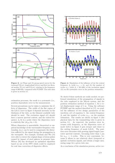
Figure 4: Simulation of the influence of (a) the central
frequency f 0 (with n cyc = 6); and (b) the number of
cycles n cyc (with f 0 = 60 kHz) of the excitation signal
s(t) on the systematic error in the position estimation.
estimation processes, the result is a systematic (i.e.,
position dependent) error in the measurement.
Several precautions can be taken to minimize the effects
of dispersion. The width of the flat region of
the L(0,1) curve in figure 3 depends inversely on the
thickness of the tube, so the thinnest available tube
should be used. The excitation signal s(t) should
have a narrow spectral content, and the central frequency
f 0 lie in a point where the dispersion curve
is relatively flat (dc ph /dω ≃ 0).
Where dispersion is unavoidable, theoretical or empirical
knowledge of the wavenumber-frequency relationship,
ξ(ω), can be used to compensate the distortion
suffered by the signal during the propagation in
the waveguide. For example, Gorham and Wu [15]
were able to restore the original shape of stress pulses
caused by impact of steel spheres in pressure bars.
Wilcox [16] has developed an optimized algorithm
based on use of the FFT which could be employed
for real time correction of dispersive effects.
To check if these methods are really needed, we performed
simulations of the propagation of signals in
the tube employed in the Micrus system, and the
position estimation method of equation 1, for a total
displacement range of 1 m. Using the software
PCDISP and the method described in [17], we studied
the influence of two design parameters of the
waveform s(t) of equation 5: the central frequency
f 0 and the number of cycles n cyc , on the position
estimation. The results are shown in figure 4 (the
physical data for the transmitting tube is given in
section 3.1. As expected, the position error increases
with frequency, as the dispersion curve of
mode L(0,1) in figure 3 gets steeper and closer to
the cutting frequency of mode L(0,2). The position
error decreases with growing signal length (narrower
spectral content), becoming lower than 1 µm
for n cyc > 4 cycles. This is very convenient, because
it allows to use relatively short (temporal or
spatial) excitation signals, and obtain a longer measuring
range for a given tube size.
As a conclusion of the simulation process, active cor-
4/8