Indoor Pedestrian Navigation using an INS/EKF framework for Yaw ...

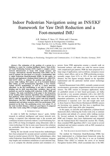
Indoor Pedestrian Navigation using an INS/EKFframework for Yaw Drift Reduction and aFoot-mounted IMUA.R. Jiménez, F. Seco, J.C. Prieto and J. GuevaraConsejo Superior de Investigaciones Científicas.Ctra. Campo Real km. 0.2; La Poveda, 28500, Arganda del Rey.Madrid (Spain).Telephone: (34) 918711900, Fax: (34) 918717050Email: arjimenez@iai.csic.esWeb: http://www.iai.csic.es/lopsiWPNC 2010: 7th Workshop on Positioning, Navigation and Communication, 11-12 March, Dresden, Germany, 2010.Abstract—The estimation of the position of a person in abuilding is a must for creating Intelligent Spaces. State-of-theartLocal Positioning Systems (LPS) require a complex sensornetworkinfrastructure to locate with enough accuracy andcoverage. Alternatively, Inertial Measuring Units (IMU) can beused to estimate the movement of a person; a methodology thatis called Pedestrian Dead-Reckoning (PDR). In this paper, wedescribe and implement a Kalman-based framework, called INS-EKF-ZUPT (IEZ), to estimate the position and attitude of aperson while walking. IEZ makes use of an Extended Kalmanfilter (EKF), an INS mechanization algorithm, a Zero VelocityUpdate (ZUPT) methodology, as well as, a stance detectionalgorithm. As the IEZ methodology is not able to estimate theheading and its drift (non-observable variables), then severalmethods are used for heading drift reduction: ZARU, HDR andCompass. The main contribution of the paper is the integrationof the heading drift reduction algorithms into a Kalman-basedIEZ platform, which represents an extended PDR methodology(IEZ+) valid for operation in indoor spaces with local magneticdisturbances. The IEZ+ PDR methodology was tested in severalsimulated and real indoor scenarios with a low-performance IMUmounted on the foot. The positioning errors were about 1% ofthe total travelled distance, which are good figures if comparedwith other works using IMUs of higher performance.I. INTRODUCTIONIn order to fulfil the Intelligent Spaces’ goals, furtherresearch in artificial intelligence and sensor network technology,is required. One important topic is the accurate andcontinuous location of persons indoors. Local Positioning Systems(LPS) are being investigated, using ultrasound, radio orvision technology [1], but in some cases beacon-free solutionsare preferable since they do not depend on a pre-installedinfrastructure.During the last decade several beacon-free methodologieshave been proposed for accurate person’s position estimationbased on inertial sensors [2]-[14]. These methodologies, oftencalled Pedestrian Dead-Reckoning (PDR) solutions, integratestep lengths and orientation estimations at each detected step,so as to compute the absolute position and orientation of aperson. Some PDR approaches assume a smooth walk onhorizontal surfaces, and others are valid for uneven terrainwith complicated gait patterns. PDR has been proposed for alarge range of applications, such as defense, emergency rescueworkers, smart offices, and so on. PDR positioning accuracy,normally ranges from 0.3% to 10% of the total travelleddistance, but this figures strongly depend on the algorithmimplemented and the particular inertial sensor technologyemployed.Inertial Measurement Units (IMU), normally contain severalaccelerometers, gyroscopes, magnetometers and even pressuresensors. The IMU sensors in aerospace applications, basedon gimballed sensors or laser based gyroscopes, are bulkybut provide a very accurate estimation with a low drift [9].The size and performance of an inertial sensor are linearlydependent parameters, so the smaller the sensor the lowerperformance is expected. Low- size and weight units suchas those based on Micro-Electro-Mechanical (MEMS) sensorsare becoming very popular, but they have a significant biasand therefore suffer large drifts after integration.In this paper, we describe and implement a Kalman-basedframework (IEZ), following the Foxlin work [14], to estimatethe position and attitude of a person while walking (sectionII). Several methods for heading Drift reduction: ZARU,HDR and Compass, have been implemented and integratedinto the Kalman-based IEZ framework (section III). Finally,these extended PDR algorithms (IEZ+) were tested in severalsimulated and real indoor scenarios with an IMU mounted onthe foot (section IV).II. THE KALMAN-BASED INERTIAL PDR METHODThe method for Pedestrian Dead-Reckoning (PDR) hasbeen implemented in a Kalman-based framework using theguidelines of Foxlin [14]. The idea is to use an ExtendedKalman Filter (EKF) to estimate the errors of an InertialNavigation System (INS), which accumulate due to the IMU

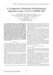
AccelerationAngular ratePositionVelocityINS for Position and Attitude estimationAttitudeError state vectorAttitudeExtended Kalman Filter (EKF) for error estimationMeasurementEvent detectionZUPTEstimated velocity3) Remove the gravitational component in accelerationreadings (3).4) Integration of acceleration values to estimate the velocityand, after a second integration, the position (4.a & 4.b).5) Refinement of position, velocity and attitude based onKalman error estimates (5.a, 5.b & 5.c).The first phase for bias compensation consists in subtractingto the raw acceleration and gyroscopic sensor data (ωk b anda b krespectively), the bias terms estimated by the Kalman filter(positions 4-6 and 13-15 in the error state vector for gyro andaccelerometers biases, respectively):AccelerationAccelerometersStance & Still phase detectionAngular rateGyroscopesFig. 1. The IEZ Kalman-based framework used for pedestrian deadreckoning.It has four main blocks: 1) an INS mechanization algorithm adaptedto incorporate the error estimations from an EKF, 2) a Extended Kalman Filter(EKF) that estimates the errors states related to the INS, 3) a Zero-Velocity-Update (ZUPT) block that feeds the EKF with the measured errors in velocity,and 4) a Stance&Still detection algorithm to determine when the person isat rest (Still) or with the foot on the ground while walking (Stance). In thisframework 3 accelerometers and 3 gyroscopes are used in an IMU mountedon the foot of a person.sensor biases. The EKF is updated with velocity measurementsby the Zero-Velocity-Update strategy (ZUPT) every time thefoot is on the floor. We call this Kalman-based frameworkINS-EKF-ZUPT, or just IEZ, for short. Figure 1 shows themain blocks in the IEZ PDR methodology.A. Inertial Navigation (INS)The INS algorithm uses the accelerometer and gyroscopicreadings, in the sensor body (b) frame of reference, (a b k andωk b , respectively) which are taken at every sample interval ∆tat discrete sampling times k. A classical INS mechanizationwas implemented, including some modifications to cope withthe information provided by the EKF throughout the errorstate vector: δx k = [δϕ k ,δωk b,δr k,δv k ,δa b k]. This 15-elementvector contains the estimated biases for accelerometers andgyroscopes (δω b and δa b , respectively), as well as, the errorsin attitude (δϕ) and the errors in position and velocity (δr,δv).All these 5 components have 3 elements each, correspondingto a three-dimensional estimation. Details of the designed INSblock for use in the IEZ framework are shown in Fig. 2 andexplained in the following.This INS mechanization process has five main phases:1) Bias compensation of raw acceleration and gyroscopicvalues based on Kalman bias estimates (1.a & 1.b inFig. 2).2) Integration of gyroscopic values in order to estimate theattitude (2).{ ω ′ bk = ωk b −δx k−1(4 : 6) = ωk b −δωb k−1= a b k −δx k−1(13 : 15) = a b k −δab k−1a ′ bk, (1)where ω ′ bkand a ′ bkdenote the bias-compensated gyroscopicand acceleration sensor readings, respectively.In the second phase, we update the sensor orientation, withrespect to the navigation frame (n, defined to be Noth-West-Up on the ground), based on the bias-compensated gyroscopicreadings. A Padé approximation of the exponential function isused for this orientation update [11]:C n b k|k−1= f(C n b k−1|k−1,ω ′ k−1|k−1·2I bk ) = C n 3×3 +δΩ k ·∆tb2I 3×3 −δΩ k ·∆t ,(2)where C n b k|k−1is the rotation matrix that transforms fromthe body (b) to the navigation (n) frame, which is updated withthe gyroscopic information at time k but not yet corrected bythe EKF; C n b k−1|k−1is the last rotation matrix available thatwas already corrected by the EKF after the filter update at timek−1; and δΩ k is the skew symmetric matrix for angular ratesused to define the small angular increments in orientation:⎡δΩ k = ⎣0 −ω ′ bk(3) ω ′ bk(2)ω ′ bk(3) 0 −ω ′ bk(1)−ω ′ bk(2) ω ′ bk(1) 0⎤⎦. (3)Note that the rotation matrix C n b k−1|k−1is post-multipliedby the term that represents the small change in orientation,since this rotation is with respect to the sensor body referenceframe (b).In the third phase, the acceleration of gravity is removedfrom the sensor readings. Initially, the accelerations, a ′ bk, aretransformed from the sensor body coordinate frame (b) to thenavigation frame (n), and then the value of g (9.8 m/s) issubtracted to the “vertical” component of acceleration:ă k = C n b k|k−1 · a ′ bk −[0,0,g]. (4)In the fourth phase, the gravity-free acceleration value ă k ,is integrated to obtain the velocity in the navigation frame,v k|k−1 , prior to the EKF correction at time k:v k|k−1 = v k−1|k−1 + ă k ·∆t. (5)

Fig. 2. Details of the INS mechanization algorithm adapted to be used in cooperation with the EKF in the IEZ framework. It accepts the estimated sensorbiases for accelerometers and gyroscopes (δω b and δa b , respectively), as well as, the errors in attitude (δϕ) and the errors in velocity and position (δr,δv).This velocity is integrated to obtain the sensor position inthe navigation frame:r k|k−1 = r k−1|k−1 + v k|k−1 ·∆t. (6)then, the linearized state transition model is:δx k+1|k = Φ k δx k|k + w k , (11)where δxFinally, in the fifth phase, we correct the previously computedposition and velocity estimates once the EKF has beenk is the process noise withk+1|k is the predicted error state, δx k|k is the lastfiltered error state at time k, wcovariance matrix Qupdated with the measurements at time k, by making use ofk = E(w k w T k ), and Φ k is the 15 × 15state transition matrix:the filtered Kalman error state δx k :{ Φrk|k = r k|k−1 −δx k (7 : 9) = r k|k−1 −δr k =k ⎡.I ∆t·C n ⎤v k|k = v k|k−1 −δx k (10 : 12) = v k|k−1 −δvb k k|k0 0 0(7)0 I 0 0 0The attitude refinement is achieved by updating the rotation⎢0 0 I ∆t·I 0matrix, C n b k|k−1, with the three angle errors estimated by the⎣ −∆t·S(a ′ n⎥∆t·Cn ⎦ .k b k|kEKF for roll, pitch and yaw (δϕ k ). Assuming that those 0 0 0 0 Iangle errors are small, the corrected rotation matrix, C n b k|k,(12)is computed, using another Padé approximation, as:The term S(a ′ nk k is the skew symmetric matrixfor accelerations that allows the EKF to act as an inclinometer,C n b k|k= g(C n b k|k−1,δϕ k ) = 2I 3×3 +δΘestimating the pitch and roll of the sensor:k· C n b2I 3×3 −δΘ k|k−1(8)⎡ ⎤k 0 −a zk a ykwhere δΘ k is the skew symmetric matrix for small anglesS(a ′ n⎣ ak zk 0 −a xk⎦. (13)⎡⎤−a yk a xk 00 −δϕ k (3) δϕ k (2)δΘ k = −⎣δϕ k (3) 0 −δϕ k (1) ⎦. (9) a ′ nk is the bias-corrected acceleration that has been transformed−δϕ k (2) δϕ k (1) 0to the navigation frame of reference:Note that the original rotation matrix has been premultipliedby the incremental rotation term since this small change ina ′ nk = C n b k|k · a ′ bk = (a xk ,a yk ,a zk ). (14)orientation is with respect to the navigation frame (n).B. The Extended Kalman filter (EKF)The PDR navigation state transition model is a non-linearfunction of the states, but it can be linearized around a stateestimate [14], [11]. If the 15-element error state vector at timek isThe measurement model isz k = Hδx k|k + n k (15)where z k is the error measurements, H is the measurementmatrix, and n k is the measurement noise with covariancematrix R k = E(n k n T k ).The filtered error state δx k|k at time k is obtained after ameasurement at time k is available, with the Kalman update

equation:δx k|k = δx k|k−1 + K k ·[m k − Hδx k|k−1 ], (16)where K k is the Kalman gain, m k is the actual error measurement,and δx k|k−1 is the predicted error state.The Kalman gain is calculated during the correction phasewith the usual formula:K k = P k|k−1 H T (HP k|k−1 H T + R k ) −1 . (17)where P k|k−1 is the estimation error covariance matrix, thatis computed at time k based on measurements received at timek-1, in this way: P k|k−1 = Φ k−1 P k−1|k−1 Φ T k−1 + Q k−1. Thecovariance matrix P k|k at time k is then computed using theKalman gain in the Joseph form equation: P k|k = (I 15×15 −K k H)P k|k−1 (I 15×15 − K k H) T + K k R k K T k . Similarly, duringthe update phase after corrections with measurements at timek, the predicted covariance matrix for time k+1 is computedas: P k+1|k = Φ k P k|k Φ T k + Q k.It is important to mention that the non-bias error terms ofthe filtered state vector, δx k|k , are reset to zero after the INSuses them to refine the current attitude, velocity and position.This is because those errors are already compensated andincorporated into the INS estimations. The only terms thatare maintained over time in the EKF filter are the gyro andaccelerometer biases, i.e. δω b k and δab k .The actual error measurement m k that feeds the EKF, iscalculated for ZUPT as: m k = v k|k−1 − [0,0,0], wherethe zero vector means that at stance we know that thevelocity of the foot is almost zero. The measurement matrix,H, for ZUPT update is a 3 by 15 matrix like this:H = [0 3×3 , 0 3×3 , 0 3×3 , I 3×3 , 0 3×3 ]. It selects the velocityerror components from the error state matrix δx k , i.e. the 10thto 12th terms.C. Stance detectionThe EKF gets feedback from measurements, only when theperson’s foot is detected to be stationary on the ground (totallystill, or in a stance phase during walk). Most algorithms in theliterature for stance detection rely on basic signal processingtechniques with accelerometers [5], [13] or gyroscopes [2].They properly work in many situations but occasionally failin slow and random walk [13]. We implement a multiconditionalgorithm, that complements the implementation of[10] by using both sources of information (accelerometers andgyroscopes) and an order filter so as to make the detectionprocess robust enough (see Fig. 3).The three conditions (C1, C2 and C3) to declare a foot asstationary are:1) The magnitude of the acceleration, |a k | = [a b k (1)2 +a b k (2)2 + a b k (3)2 ] 0.5 must be between two thresholds(th amin = 9 and th amax = 11 m/s 2 ).C1 ={1 thamin < |a k | < th amax0 otherwise. (18)Stance & Still phase detectionC1: Magnitude of acceleration conditionC2: Local variance of acceler. conditionC3: Angular rate conditionFig. 3.AccelerationIMUAngular rateAND Median filter Stance & StilldetectionEvent detectionSetup measurement for EKFStance and Still detection block used in the IEZ framework.2) The local acceleration variance, which highlights thefoot activity, must be above a given threshold (th σa =3 m/s 2 ). The local variance is computed this way:σ 2 a b k= 12s+1k+s∑j=k−s(a b k −a b k )2 , (19)where a b kis a local mean acceleration value, computedby this expression:a b k = 1 ∑ k+s2s+1 q=k−s a q, andsdefinesthe size of the averaging window (s = 15 samples). Thesecond condition C2 is satisfied when:C2 ={ 1 σa bk> th σa0 otherwise. (20)3) The magnitude of the gyroscope, |ω k | = [ω b k (1)2 +ω b k (2)2 + ω b k (3)2 ] 0.5 , must be below a given threshold(th ωmax = 50 o /s).C3 ={ 1 |ωk | < th ωmax0 otherwise. (21)The three logical conditions must be satisfied simultaneouslyfor foot stationary detection, so a logical “AND” isapplied, and the result is filtered out using a median filter witha neighboring window of 11 samples in total. The registeredlogical “1”s mark the Stance phase that occurs when the foot isstationary on the floor (while walking, or not). The Still phase,corresponding to a non-walking stationary foot, is detectedfrom stance samples that are not surrounded by non-stancesamples in a window larger than 2 seconds. Figure 4 showsresults of this multi-condition stance detection process.III. METHODS TO REDUCE THE DRIFT IN HEADINGThe IEZ Kalman-based PDR method presented in lastsection (Fig. 1), accumulates large errors in orientation dueto the bias in the gyroscopes. IEZ can not estimate it becausethe yaw orientation (ψ k ), and the gyroscopic bias (δω b ) in thevertical axis, are not observable from ZUPT measurementsalone [14]. Next subsections describe the integration in IEZof some approaches to reduce the drift in heading: ZARU[10], HDR [12], and the use of magnetometers as a compass.We focus on methods to reduce the drift without usingany external infrastructure such as GPS and LPS, nor mapmatchingtechniques. See Fig. 5 to view how these methodsare integrated in the IEZ framework.

Logical (0−1 with added offsets)54Conditions for Stance & Still state detectionCond1Cond2Cond3Stance = C1&C2&C3StancemedianStill(no − walk)Steps detected32101200 1400 1600 1800 2000 2200 2400 2600 2800samplesFig. 4. Some results of the Stance and Still detection process.A. Zero angular rate update (ZARU)ZARU stands for Zero Angular Rate Update [10]. So, theidea is to feed the EKF with measurements of the measurederror in the angular rate, while the foot is still.∆ωk b = ωb k −[0,0,0]. (22)If ZARU is integrated in the IEZ framework, then itsmeasurement matrix must be:[ ]03×3 IH = 3×3 0 3×3 0 3×3 0 3×3, (23)0 3×3 0 3×3 0 3×3 I 3×3 0 3×3and the error measurement vector is the concatenation ofthe ZARU and ZUPT contributions:B. Heuristic Heading Reduction (HDR)m k = [∆ω b k ,∆v k]. (24)HDR stands for Heuristic Heading Reduction. It was originallyproposed by Borestein et al. [12]. It makes use of the factthat many corridors or paths are straight. So, the idea of theHDR algorithm is to detect when a person is walking straight,and in that case apply a correction to the gyro biases, in orderto reduce the heading error.In our paper we use the same hypothesis, but we implementit in a total different way as Borestein et al. did [12]. Insteadof filtering the gyro signals with a binary I-controller, we workin the Yaw space, detecting a straight walk by analyzing theorientation change, ∆ψ k , among successive steps:∆ψ k = ψ k − ψ k−(k s−k s−1) +ψ k−(ks−k s−2), (25)2where ψ k is the heading of the foot at the current samplek computed as ψ k = arctan(C n b k|k(2,1), C n b k|k(1,1)); k s isthe sample of last detected step (red points in Fig. 4), andk s−1 is the sample of the previous to the last detected step.The right part of equation 25 takes the average of two Yawvalues at positions within the previous stance phases that arecorrelative with the position of sample k in its own stancephase.If the orientation change among successive steps, ∆ψ k , issmall enough (below a given threshold), then it is assumed astraight-line walk; and the EKF is fed with some measurement,m k , to correct the heading error so as to make the trajectorystraight:Fig. 5. The IEZ-extended PDR framework. It represents the same methodologyas presented in Fig. 1 but adding the blocks for heading drift reduction:ZARU, HDR and Compass.m k ={∆ψk |∆ψ k | ≤ th ∆ψ0 otherwise, (26)If |∆ψ k | is larger than th ∆ψ , then the orientation change isconsidered to be a real variation in the trajectory of a person.In that case, no corrections are fed into the EKF. We use anangular value of 4 degrees as threshold th ∆ψ .The measurement matrix, H, when incorporating the ZUPTand HDR updates is a 4 by 15 matrix as follows:[ ][001] 01×3 0H =1×3 0 1×3 0 1×3. (27)0 3×3 0 3×3 0 3×3 I 3×3 0 3×3

C. Electronic CompassThis drift compensation method is normally used in outdoorenvironments, where magnetic disturbances are moderate. Indoors,the magnetic disturbances can be severe and permanentfor a given position of the user. Some authors [12] do notrecommend the use of magnetometers indoors, but, convenientlytreated, we believe they are very useful as an absolutereference for heading.In order to use the magnetometer sensor as a compass, wefirst transform the sensor body readings into the navigationframe of reference, using the Roll (φ k ) and Pitch (θ k ) angles:⎡B n k = ⎣ cosθ ⎤ ⎡k 0 −sinθ k0 1 0 ⎦· ⎣ 1 0 0 ⎤0 cosφ k −sinφ k⎦·B b k ,−sinθ k 0 cosθ k 0 sinφ k cosφ k(28)where the roll and pitch angles are obtained from the rotationmatrix, as follows: φ k = arctan(C n b k|k(3,2), C n b k|k(3,3))and θ k = −arcsin(C n b k|k(3,1)).After this transformation, the magnetic field components aregeodetically levelled, so the heading angle (ψcompass k) is:ψcompass k= −arctan(B n k(2)/B n k(1))−M d (29)where M d is the earth magnetic declination at a given pointon the earth surface.The compass error measurement m k for the EKF ism k = ∆ψ k = ψ k −ψcompass k. (30)The measurement matrix, H, for ZUPT and Compass estimationis equal to the HDR case (eq. 27).D. The full integration of all methods in IEZOnce defined each individual method for drift reduction(ZUPT, ZARU, HDR and Compass), the evaluation of allthese methods merged into the same IEZ framework is quitestraightforward. The measurement matrix would be a 8 by 15matrix with these components:⎡⎤0 3×3 0 3×3 0 3×3 I 3×3 0 3×3H = ⎢ 0 3×3 I 3×3 0 3×3 0 3×3 0 3×3⎥⎣ ⌊001⌋ 0 1×3 0 1×3 0 1×3 0 1×3⎦ , (31)⌊001⌋ 0 1×3 0 1×3 0 1×3 0 1×3and the measurement vector would be:m k = [∆v k ,∆ωk,∆ψ b HDR k ,∆ψ Compassk]. (32)IV. TESTSWe have performed several tests in order to evaluatethe performance of these PDR methods: IEZ, IEZ+ZARU,IEZ+HDR, IEZ+Compass and IEZ+ZARU+HDR+Compass.Some tests were performed by simulation, but most of thembelong to real indoor scenarios, where the IMU is installed onthe right foot of a person, as Fig. 6 shows.Fig. 6.Xsens IMU attached to the right foot using the shoe’s laces.accelerometers gyroscopes magnetometersAxes 3 3 3Full Scale (FS) ±50 m/s 2 ±300 deg/s ±750 mGaussLinearity 0.2% of FS 0.1% of FS 0.2% of FSBias stability 0.02 m/s 2 1 deg/s 0.1 mGaussBandwidth 30 Hz 40 Hz 10 HzMax update rate 512 Hz 512 Hz 512 HzTABLE IPERFORMANCE OF INDIVIDUAL SENSORS IN XSENS IMUA. IMU descriptionWe use a commercially available IMU, model MTi fromXsens Technologies B.V (Enschede, The Netherlands). Its sizeis 58x58x22 mm (WxLxH), and it weights 50 grams. It isconfigured to send data at 100 Hz.The IMU has three orthogonally-oriented accelerometers,three gyroscopes and three magnetometers. The accelerometersand gyroscopes are MEMS solid state with capacitativereadout, providing linear acceleration and rate of turn,respectively. Magnetometers use a thin-film magnetoresistiveprinciple to measure the earth magnetic field.The performance of each individual MEMS sensor withinthe MTi IMU are summarized in table I. They suffer froma significant bias, and this bias also varies over time, soPDR algorithms have the challenge of avoiding excessive erroraccumulation (drift) during integration.B. EKF TuningThe EKF in the IEZ and the extended IEZ+ frameworkshad to be fine-tuned in order to obtain a stable operation, byselecting the values of matrixes Q k , R k and P k|k−1 .The process noise covariance matrix, Q k , is initialized fork = 1 as a diagonal 15x15 matrix with these in-diagonalelements: [1·10 −41×3 rad,0 1×3,0 1×3 ,1·10 −41×3 m/s,0 1×3]. Thenon-zero values correspond to the variance of gyroscopic andaccelerometer sensors that is, in both cases, about 1·10 −4 .The measurement noise covariance matrix: R k is a squarematrix with rows and columns equal to the number, n, ofmeasurements available (3 for ZUPT, 4 for IEZ+ZARU, 6 for

6050Real traj.IEZIEZ ZARUIEZ HDR0.01State vector [4:6]: Gyro bias40IEZ CompassIEZ Compass+HDR+ZARUStart0−0.01North (m)30−0.02δω b k (1)δω b k (2)20−0.03δω b k (3)10−0.040−0.05−40 −30 −20 −10 0 10 20 30East (m)Fig. 7. Estimated trajectories from IEZ PDR algorithms, when using IMUsimulated data.IEZ+HDR, 7 for IEZ+ZARU+HDR, and so on). We set thismatrix with in-diagonal elements with values of: 0.01 m/s forZUPT, 0.1 rad/s for ZARU, and 0.1 rad HDR and Compass.The state estimation covariance matrix, P k|k−1 , is initializedas a diagonal 15x15 matrix with these in-diagonal elements:[0 1×3 ,1·10 −21×3 rad/s,0 1×3,0 1×3 ,1·101×3 −2 m/s2 ].The results of the PDR algorithms strongly depends on theselected values for these covariance matrixes, so the tuningmust be done trying to find a consistent response among thestate estimates and the state estimation covariance matrix.C. Performance using simulated IMU dataWe simulated the data an IMU would output when a personis walking along a pre-defined trajectory and the IMU ismounted on the foot. This simulator was useful to better tunethe EKF, and also to add controlled noise and biases to anyof the simulated sensors.A square trajectory of 20-meters-long side was simulatedwith a velocity of 1 m/s and a constant stride length of 1 meter.The gyroscopic biases were zero for X and Y axis, but wasset to -0.05 rad/s in Z axis. Additionally, white Gaussian noisewith zero mean was added to the accelerometer and gyroscopicsamples (σ a = 0.01 m/s 2 and σ ω = 0.01 rad/s). Figure 7shows the positioning results using the IEZ and the differentIEZ-extended algorithms. It is clear how a heading drift isaccumulated due to the gyro bias using the IEZ method alone.However, we can see how the addition of several headingrelatedmeasurements to IEZ (ZARU+HDR+Compass) givesbetter results that in any other cases.The estimation of the gyroscopic bias in the Z axis, usingany of the IEZ+ extended methods, gets stable after 5 seconds(500 samples), as can be seen in Fig. 8. This initial periodcorresponds to the Still phase, just before the person startsto walk. Once the person is walking, the gyroscopic biasestimation is no longer changed since the state estimationcovariance matrix converged to low values, which means thatthe bias estimation was reliably done.0 500 1000 1500 2000 2500 3000 3500 4000samplesFig. 8. Simulation of the evolution of the gyroscopic biases as estimatedby the EKF in any of the IEZ+ extended methods. The vertical gyro biasconverges in a few seconds to the true bias value (-0.05 rad/s).North (m)555045403530252015105Real traj.IEZIEZ ZARUIEZ HDRIEZ CompassIEZ Compass+HDR+ZARU0 10 20 30 40 50 Start 60East (m)Fig. 9. Position estimation results using IEZ and several IEZ-extended PDRalgorithms. The test is performed in building A of IAI-CSIC campus in aCounter-Clock-Wise (CCW) direction. The path is about 125 meters long,and it contains indoor as well as outdoor parts.D. Performance in real indoor environmentsWe tested the PDR algorithms in a real indoor environment.Tests were performed in building “A” of IAI-CSIC campus,both in a Counter-Clock-Wise (CCW) and Clock-Wise (CW)directions. Figures 9 and 10 show the estimated trajectoriesfor a path 125 meters long, completed in 100 seconds.It is important to mention that the Compass contribution isdecisive in order to obtain accurate trajectories with respectthe ideal path. This is valid even with several local magneticperturbations that were detected along the path, as can be seenin Fig. 11.As an initial performance index, we computed the positioningerrors (difference between the initial and final position)with respect to the total travelled distance (TTD). The values

North (m)555045403530252015105Fig. 10.a.u.21.510.50Real traj.IEZIEZ ZARUIEZ HDRIEZ CompassIEZ Compass+HDR+ZARU0 10 20 30 40 50 Start 60East (m)The same test than in figure 9 but in Clock-Wise (CW) direction.Magnetic Fieldm xm ym z|m|V. CONCLUSIONWe have described, implemented and compared some ofthe most relevant Kalman-based PDR algorithms in the stateof the art for pedestrian dead reckoning. The study consistedin the implementation of several methods for heading driftreduction, and the evaluation in a common IEZ PDR platform.We restricted the study to the use of an IMU sensor alone, i.e.without using any external infrastructure such as GPS, LPSor building-maps to correct the heading drift. The device wasplaced at the foot of the person because is the best positionfor accurate PDR.The presented results shown that extended IEZ+ PDRalgorithms can provide good solutions for estimating humantrajectories, even in indoors environments with local magneticdisturbances, and even using a low-performance IMU. The uncorrectedheading drift is proportional to the travelled distancebut not to the time elapsed. The positioning error, for the IEZ+method integrating ZARU+HDR+compass, is typically about1% of the total travelled distance.Future work will be focused to obtain a periodic absolutepositioning update during the walk, in order to cancel outany drift. This update could be done with LPS sensors suchas those based on RFID, WiFi, UWB or ultrasound; alsomatching PDR estimations with local maps; or using any kindof magnetic signatures that can be associated to a knownposition. Any of these approaches should provide a betterindoor location of persons for Intelligent Spaces in scenariossuch as homes, offices, healthcare spaces, emergencies, sportcenters and so on.−0.5−10 1000 2000 3000 4000 5000 6000 7000 8000 9000 10000samplesFig. 11. Magnetometer readings, B b k (for k=1 to 10000), during thewalking test in the indoor environment of Fig. 9. Note that the magnetic fieldmagnitude is not constant along the path due to local magnetic disturbances.presented in table II show the typical range of positioningerrors found for several indoor tests like those presented infigures 9 and 10.PDR MethodPositioning errors (% of TTD)IEZ > 15IEZ ZARU [4-8]IEZ HDR [2-10]IEZ Compass [0.6-5]IEZ ZARU+HDR+Compass [0.3-1.5]TABLE IITYPICAL PERFORMANCE OF IEZ AND IEZ+ PDR ALGORITHMS FORSEVERAL INDOOR TESTS. ERRORS IN PERCENTAGE OF TOTAL TRAVELLEDDISTANCE (TTD).ACKNOWLEDGMENTThe authors would like to thank the financial supportprovided by projects LEMUR (TIN2009-14114-C04-03),RESELAI (TIN2006-14896-C02-02) and LOCA (CSIC-PIERef.200450E430).REFERENCES[1] A.R. Jiménez, F. Seco, C. Prieto, and J. Roa, “Tecnologías sensorialesde localización para entornos inteligentes,” in I Congreso español deinformática - Simposio de Computación Ubicua e Inteligencia Ambiental,UCAmI2005 (Granada), 2005, pp.75-86.[2] R. Feliz, E. Zalama and J. Gómez, “Pedestrian tracking using inertialsensors,” Journal of Physical Agents, vol. 3 (1), pp. 35-42, 2009.[3] B. Beauregard, “Omnidirectional Pedestrian Navigation for First Responders,”in 4th Workshop on Positioning, Navigation and communication,WPNC’07, Hannover, 2007, pp. 33-36.[4] J. Won Kim, H.J. Jang, D. Hwang and C. Park, “A step, stride and headingdetermination for the pedestrian navigation system,” Journal of GlobalPositioning Sustems, vol. 3 (1-2), pp.273-279, 2004.[5] R. G. Stirling, “Development of a pedestrian navigation system usingshoe mounted sensors”, Master of Science, University of Alberta, 2003.[6] R Stirling, J. Collin, K. Fyfe and G. Lachapelle, “An Innovative ShoemountedPedestrian Navigation System”, In GNSS 2003, Graz, Austria,22-25 April, 2003, pp. 1-15.[7] H. Weinberg, “Using the ADXL202 in Pedometer and Personal NavigationApplications,”Analog Devices AN-602 application Note, 2002[8] T.J. Brand and R.E. Phillips, “Foot-toFoot Range Measurement as anAid to Personal Navigation,´´ in ION 59th Annual Meeting, 23-25 June,Alburquerque, NM, 2003, pp. 113-121.

[9] L. Ojeda and J. Borestein, “Non-GPS Navigation for Emergency Responders,”In International joint Topical Meeting on Sharing Solutions forEmergencies and Hazardous Environments, February 12-15, Salt LakeCity, Utath, USA, 2006, pp. 1-8.[10] S. Rajagopal, “Personal dead reckoning system with shoe mountedinertial sensors,” In Master of Science Thesis, Stockholm, Sweeden, 2008,pp. 1-45.[11] A. Schumacher, “Integration of a GPS aided Strapdown Inertial navigatiosystem for land vehicles,” In Master of Science Thesis, Stockholm,Sweeden, 2006, pp. 1-57.[12] J. Borestein, L. Ojeda and S. Kwanmuang, “Heuristic reduction of gyrodrift in IMU-based personnel tracking system,” In SPIE Defense, Securityand Sensing Conference, April 13-17, Orlando, Florida, USA, 2009, pp.1-11.[13] A.R. Jiménez, F. Seco, C. Prieto and J. Guevara, “A Comparison ofPedestrian Dead-Reckoning Algorithms using a Low-Cost MEMS IMU,”In 6th IEEE International Symposium on Intelligent Signal Processing,26-28 August, Budapest, Hungary, 2009, pp. 37-42.[14] E. Foxlin, “Pedestrian tracking with shoe-mounted inertial sensors,”IEEE Computer graphics and Applications, vol. 1, pp. 38-46, 2005.