A High Accuracy Magnetostrictive Linear Position Sensor

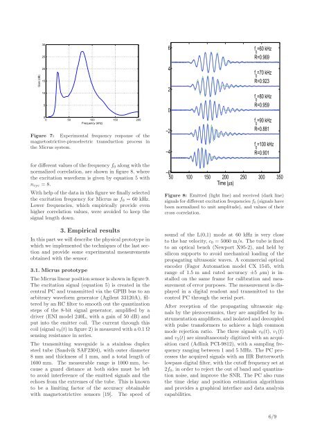
Gain (dB)3025201510500 50 100 150 200Frequency (kHz)Figure 7: Experimental frequency response of themagnetostrictive-piezoelectric transduction process inthe Micrus system.6420−2−4f =60 kHz0R=0.969f =70 kHz0R=0.923f =80 kHz0R=0.959f =90 kHz0R=0.881f =100 kHz0R=0.901for different values of the frequency f 0 along with thenormalized correlation, are shown in figure 8, wherethe excitation waveform is given by equation 5 withn cyc = 8.With help of the data in this figure we finally selectedthe excitation frequency for Micrus as f 0 = 60 kHz.Lower frequencies, which empirically provide evenhigher correlation values, were avoided to keep thesignal length down.3. Empirical resultsIn this part we will describe the physical prototype inwhich we implemented the techniques of the last sectionand provide some experimental measurementsobtained with the sensor.3.1. Micrus prototypeThe Micrus linear position sensor is shown in figure 9.The excitation signal (equation 5) is created in thecentral PC and transmitted via the GPIB bus to anarbitrary waveform generator (Agilent 33120A), filteredby an RC filter to smooth out the quantizationsteps of the 8-bit signal generator, amplified by adriver (ENI model 240L, with a gain of 50 dB) andput into the emitter coil. The current through thiscoil (signal v 0 (t) in figure 2) is measured with a 0.1 Ωsensing resistance in series.The transmitting waveguide is a stainless duplexsteel tube (Sandvik SAF2304), with outer diameter8 mm and thickness of 1 mm, and a total length of1600 mm. The measurable range is 1000 mm, becausea guard distance at both sides must be leftto avoid interference of the emitted signals and theechoes from the extremes of the tube. This is knownto be a limiting factor of the accuracy obtainablewith magnetostrictive sensors [19]. The speed of−650 100 150 200 250 300 350Time (µs)Figure 8: Emitted (light line) and received (dark line)signals for different excitation frequencies f 0 (signals havebeen normalized to unit amplitude), and values of theircross correlation.sound of the L(0,1) mode at 60 kHz is very closeto the bar velocity, c 0 = 5060 m/s. The tube is fixedto an optical bench (Newport X95-2), and held bysilicon supports to avoid mechanical loading of thepropagating ultrasonic waves. A commercial opticalencoder (Fagor Automation model CX 1545, withrange of 1.5 m and rated accuracy ±5 µm) is installedon the same frame for calibration and measurementof error purposes. The measurement is displayedin a digital readout and transmitted to thecontrol PC through the serial port.After reception of the propagating ultrasonic signalsby the piezoceramics, they are amplified by instrumentationamplifiers, and isolated and decoupledwith pulse transformers to achieve a high commonmode rejection ratio. The three signals v 0 (t), v 1 (t)and v 2 (t) are simultaneously digitized with an acquisitioncard (Adlink PCI-9812), with a sampling frequencyranging between 1 and 5 MHz. The PC processesthe acquired signals with an IIR Butterworthlowpass digital filter, with the cutoff frequency set at2f 0 , in order to reject the out of band and quantizationnoise, and improve the SNR. The PC also runsthe time delay and position estimation algorithmsand provides a graphical interface and data analysiscapabilities.6/9