16. Sediment Transport Across the Continental Shelf and Lead-210 ...

16. Sediment Transport
Across the Continental Shelf
and Lead-210 Sediment
Accumulation Rates
William Wilcock
OCEAN/ESS 410
Lecture/Lab Learning Goals
• Know the terminology of and be able to sketch
passive continental margins
• Differences in sedimentary processes between active
and passive margins
• Know how sediments are mobilized on the
continental shelf
• Understand how lead-210 dating of sediments works
• Application of lead-210 dating to determining
sediment accumulation rates on the continental shelf
and the interpretation of these rates - LAB
Passive Margins
Terminology
Shelf Break
Abyssal Plain
Transition from continental to oceanic crust
with no plate boundary.
Formerly sites of continental rifting
Continental Shelf - Average gradient 0.1°
Shelf break at outer edge of shelf at 130-200 m depth (130 m depth = sea
level at last glacial maximum)
Continental slope - Average gradient 3-6°
Continental rise (typically 1500-4000 m) - Average gradient 0.1-1°
Abyssal Plain (typically > 4000 m) - Average slope

Active Margins
Sediment transport differences
Plate boundary (usually convergent)
Narrower continental shelf
Plate boundary can move on geological time
scales - accretion of terrains, accretionary prisms
Active margins - narrower shelf, typically have a higher sediment supply,
earthquakes destabilize steep slopes.
Sediment Supply to Continental Shelf
• Rivers
• Glaciers
• Coastal Erosion
Sediment Mobilization - 1. Waves
Sediment Transport across the Shelf
Once sediments settle on the seafloor, bottom
currents are required to mobilize them.
• Wave motions
• Ocean currents
The wave base or maximum depth of wave motions is about one half the
wave length
2

Shallow water waves
Wave particle orbits flatten out in shallow water
Wave generated bottom motions
• strongest during major storms (big waves)
• extend deepest when the coast experiences long wavelength swell from
local or distant storms
Sediment Mobilization 2. Bottom Currents
• The wind driven ocean
circulation often leads to
strong ocean currents
parallel to the coast.
• These interact with the
seafloor along the
continental shelf and
upper slope.
• The currents on the
continental shelf are
often strongest near
outer margins
Aguihas current off east coast of southern Africa. The
current flows south and the contours are in units of cm/s
Sediment Distribution on the
Continental shelf
Coarse grained sands - require strong
currents to mobilize, often confined to
shallow water where wave bottom
interactions are strongest (beaches)
Fine grained muds - require weaker
currents to mobilize, transported to
deeper water.
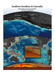
Upcoming lab
In the lab following this lecture you are
going to calculate a sedimentation rate for
muds on the continental shelf using
radioactive isotope Lead-210 and you are
going to interpret a data set collected off
the coast of Washington.
3

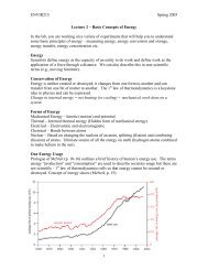
Radioactive decay - Basic equation
The number or atoms of an unstable isotope elements
decreases with time
! dN
dt
! dN
dt
" N N - Number of atoms of an
unstable isotope
= "N
T 12
= ln 2
!
λ - radioactive decay constant is
the fraction of the atoms that
decay in unit time (e.g., yr -1 )
T 1/2 - half life is the time for half
the atoms to decay
Activity - Definition and equations
A
Activity is the number of disintegrations in
unit time per unit mass (units are decays
per unit time per unit mass. For 210 Pb the
usual units are dpm/g = decays per
minute per gram )
A = c!N
! dA
dt = " A Obtained by multiplying both sides of the
C - detection coefficient, a value between
0 and 1 which reflects the fraction of the
disintegrations are detected (electrically or
photographically)
middle equation on the previous slide by
the constant cλ
238
U Decay Series
210
Pb or Pb-210 is an isotope of lead that forms as part of a decay sequence
of Uranium-238
238
U 234 U … 230 Th 226 Ra
Half Life 4.5 Byr
Rocks
Half life 1600 yrs,
eroded to
sediments
222 Rn… 210 Pb… 206 Pb
Gas, half life
3.8 days
Half life,
22.3 years
Stable
4

210-Pb in sediments
Sediments contain a background level of 210 Pb that is
supported by the decay of 226 Ra (radium is an alkali
metal) which is easily eroded from rocks and incorporated
into sediments. As fast as this background 210 Pb is lost by
radioactive decay, new 210 Pb atoms are created by the
decay of 226 Ra.
Young sediments also include an excess or unsupported
concentration of 210 Pb. Decaying 238 U in continental rocks
generates 222 Rn (radon is a gas) some of which escapes
into the atmosphere. This 222 Rn decays to 210 Pb which is
then efficiently incorporated into new sediments. This
unsupported 210 Pb is not replaced as it decays since the
radon that produced it is in the atmosphere.
Measurements of how the excess 210 Pb decreases with
depth can be used to determine rates.
Depth, Z
(or age)
Pb-210 concentrations in sediments
A B
Pb-210 activity
Region of radioactive
decay.
Background Pb-210 levels from
decay of Radon in sediments
(supported Pb-210)
Surface mixed layer - bioturbation
Measured Pb-210 activity
Excess Pb-210 activity
(measured minus
background)
t 1
t 2
Age of
sediments, t
Excess Pb-210 concentrations
A 2 A 1
Excess Pb-210 activity
Work with data in this region
For a constant
sedimentation rate, S
(cm/yr), we can
replace the depth
axis with a time axis
z = St
t = z S
! dA
dt = " A
A 2
Solving the equation - 1
" ! dA = # dt
A
A 1
t 2
"
t 1
A
"# ! ln A$ 2
% A1
= & " # t $ t 2
% t1
The equation relating activity to the
radioactive decay constant
Integrating this with the limits of
integration set by two points
! ln A 2
+ ln A 1
= ln A 1
= "( t
A 2
! t 1 )
2
A relationship between age and activity
5

Solving the equation - 2
( )
( )
ln A 1
= ! t
A 2
" t 1
2
( t 2
! t 1 ) = z ! z 2 1
S
( )
ln A 1
= ! z " z 2 1
A 2
S
( )
S = ! z 2 " z 1
ln A 1
A 2
Substitute in the relationship between
age and depth
An expression for
the sedimentation
rate
Pb-210 sedimentation rates
Plot depth against natural logarithm of Pb-210 activity
ln(A)
Depth, z
Slope = ! S "
Ignore data with background levels
Ignore data in mixed layer
Summary - How to get a sedimentation rate
1. Identify the background (supported) activity A B - the value
of A at larger depths where it is not changing with depth.
2. Subtract the background activity from the observed activities
at shallower depths and take the natural logarithm to get ln
(A)=ln(A observed -A B )
3. Plot depth z against ln(A).
4. Ignore in the points in the surface mixed region where ln(A)
does not change with depth.
5. Ignore points in the background region at depth
(A observed = A B ).
6. Measure the slope in the middle region (take it as a positive
value).
7. Multiply the slope by the radioactive decay constant (λ =
0.0311 yr -1 ) to get the sedimentation rate.
Limitations
• Assumption of uniform sedimentation
rates. Cannot use this technique
where sedimentation rate varies with
time (e.g., turbidites).
• Assumption of uniform initial and
background Pb-210 concentrations
(reasonable if composition is constant).
6