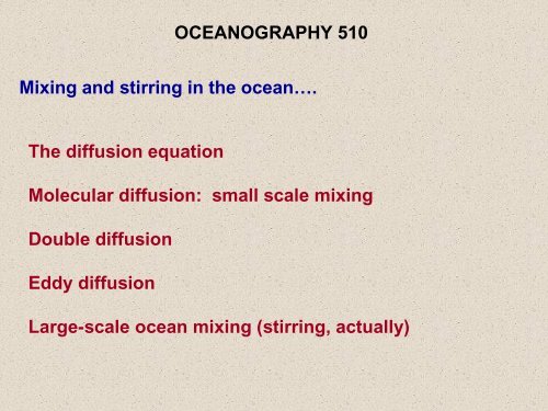
Mixing and stirring in the ocean…. The diffusion equation Molecular ...

OCEANOGRAPHY 510Mixing and stirring in the ocean….The diffusion equationMolecular diffusion: small scale mixingDouble diffusionEddy diffusionLarge-scale ocean mixing (stirring, actually)

Diffusion: basic questions….clear fluid + red dye = pink waterForward problem: describe mixingInverse problem: describe circulation[initial value problem?]What is mixing? What is stirring?

The diffusion equation….δzF x1F x2M[Flux in, x] [Flux out, x]δyδxzy∂M∂t= Flux in −Flux outx

The diffusion equation….∂M = [ F δx1 y δ z − F δx2 y δ z ] + [ F δy1 x δ z − F δy2x δ z ]∂t+ [ F δxδy−F δxδy]z1 z21 ∂M ( F (1 2)1 2)x− F Fx y− Fy( Fz1−Fz2)= + +δxδyδz ∂t δx δy δz1 ∂M ∂C= −∇ ⋅ F =V ∂t ∂t[C = concentration]

The diffusion equation….1 ∂M ∂C= −∇ ⋅ F =V ∂t ∂tchange of concentration of C inside the cubedivergence of the flux through the cubeIt is necessary to relate the concentration C tothe flux F in order to make further progress.

The diffusion equation….(i) Flux due to advection, F ASuppose the velocity vector at the center of thecube is u = (u, v, w). Then the advective flux of Cthrough the cube is uC .Check the units:⎡L⎤⎡amount of stuff ⎤ ⎡amount of stuff ⎤F A = uC ~ ⎢=3 2⎣T⎥⎢ ⎦⎣ L ⎥⎦⎢⎣ LT ⎥⎦[the units of a flux]

The diffusion equation….The complete diffusion equation becomes∂C∂t= −∇ ⋅ ( F + F ) = −∇ ⋅ ( uC)+ κ∇CA D or∂ C +∇⋅ ( uC)= κ ∇∂t2C2

The diffusion equation….Assuming that the fluid is incompressible,∇⋅ ( uC) = C∇⋅ u+ ( u⋅∇ ) C = ( u⋅∇)C ∂C ∂C ∂C= u + v + w∂x ∂y ∂zSo the diffusion equation becomesdCdt2= κ∇ C + sources & sinks

Molecular diffusion….Laminar motion: smooth and direct flow,weak inertia, relatively viscousTurbulent motion: confused flow, indirect,strong inertia, relatively inviscidLaminar motion:molecular diffusionDiffusivities are known.(see tables)κ T = 10 -3 cm 2 /secκ s = 10 -5 cm 2 /secκ u = 10 -2 cm 2 /sec ≡ νA measure of the relative size of viscous and inertialforces is the Reynolds number (Re), given byReinertial forcesviscous forces2⋅∇ ⎛U⎞ ⎛υU⎞ 2 ⎜ ⎟ ⎜ 2 ⎟u u UL= =υ∇ u ⎝ L ⎠ ⎝ L ⎠ υ

Molecular diffusion….Re = Reynolds number = inertial/viscous = UL/υLaminar flows: low ReTurbulent flows: high ReExperimentally, it has been found that the transitionbetween these states occurs around Re ~ 3000.[ 2000 – 4000 ]Re ~ UL/υ ≤ 3000 → L ≤ (3000υ)/U = (3000)(0.01)/3L ≤ 10 cmcm 2 /secOn scales of a few centimeters or less, the flow is laminar,with property gradients smoothed by molecular diffusion.On larger scales, the flow is turbulent, with propertygradients smoothed by eddy diffusion.cm/sec

Example: molecular diffusion associated with thestratification of the ocean....The ocean is stratified in both temperature and salinity,which can lead to some unexpected difffusive effects.This is known as double diffusion.Consider 3 distinct cases:(i) Warm, fresh water overlying cold, saline water.zIn the absence of any forcing,T and S gradients will diffuseaway and the ocean will becomehomogenized (both gradientsare stable).ST

Molecular diffusion….(ii) Warm, saline water overlying cold, fresh water.T is stablizing,S is destabilizing.If T stratification is initiallystronger, no direct convectionis possible.Suppose there is some length scale L associated withthe stratification, and a diffusive time scale τ.2 2L L τTκSκ ⇒ τ ⇒ 10τ κ τ κSzTTS−2

Molecular diffusion….2 2L L τTκSκ ⇒ τ ⇒ τ κ τ κST10−2Result: T gradients will diffuse away in 1% of thetime required to diffuse the S gradients. The remainingS gradient will be unstable, and overturning will occur.This phenomenon is known as salt fingering.

An example ofdouble diffusion(fingering)produced in alaboratory, takenfrom Turner,Buoyancy Effectsin Fluids.50 cm

Fingering on an interface (from Turner)2.5 cm

The horizontal structureof laboratory salt fingers,from Turner, BuoyancyEffects in Fluids.5 cm

(iii) Cold, fresh water overlying warm, saline water.zS is stabilizing,T is destabilizing.SThe T stratification will disappearfirst. If the T gradient is strongenough, overturning might occur.Eventually molecular diffusionwill remove the salinity gradient.T

Turbulent diffusion….Turbulent flows are irregular and confused.The ocean is turbulent on all scales larger than a few cm.It is still possible to use the diffusion equation(flux/gradient arguments might still hold), but we canno longer use the molecular diffusivities.The concept of a turbulent diffusivity is only aparameterization of the turbulence; essentiallywe are replacing the molecular value with a muchlarger one, but assuming the process of diffusiongenerally remains the same.[the “eddy diffusivity”]

Turbulent diffusion….Eddy diffusivities are usually many orders ofmagnitude larger than their molecular counterparts.Example: temperature in water (molecular) ~ 10 -3 cm 2 /secVertical diffusion in the ocean, κ z ~ 0.01 – 1 cm 2 /secHorizontal diffusion in the ocean, κ x ~ 10 6 – 10 8 cm 2 /secNote: in the turbulent case the eddy diffusivities might bedifferent in different directions, since the processesresponsible for the mixing might differ along coordinate axes.Example: stratification is different vertically and horizontallyin the ocean.

Turbulent diffusion….[note: for variable κ x this is∂∂x⎛⎜κx⎝∂C∂x⎞⎟⎠etc.]dCdt=∂2∂2∂2κ∇ 2C → κ + κ + κx 2 y 2 z 2[laminar]C C C∂x ∂y ∂z[turbulent]The diffusivity is now a tensor instead of a scalar.

Turbulent diffusion….The full time-dependent, nonlinear, turbulent diffusionequation has no general solution. Instead, considersome tractable problems that have been simplified.Example: Munk’s model of the oceanic thermocline.Steady; only vertical diffusion is allowed; uniformupwelling is present.upward advectionof cold waterfrom below∂T∂Tw∂ z= κz2z2∂>0 >0 >0 >0downwarddiffusion of heatfrom above[see Munk, “Abyssal recipes”, 1966]

Turbulent diffusion….∂T∂T2w∂ z= κzz2∂→2d T ⎛ w ⎞dT− ⎜ ⎟ =dz ⎝ ⎠02κ dzz[if w and κ z are constants]The solution to this ODE is of the formzT(z)( ) ( )e( w / κz) zT z = T − T + TS D DT Ssurface temperaturedeep temperatureT D

Turbulent diffusion….z/zoS D D oT( z) = ( T − T )e + T , z =κzwIn recent years κ z has been found to be ~ 0.1 cm 2 /secover much of the ocean interior. For the N. Pacific,the scale height z o can be taken to be ~ 600 m.This suggests that w ~ (0.1)/(6x10 4 ) ~ 10 −6 cm/sec .[small and unmeasurable]

Measuring turbulent diffusion….In 1993, Ledwell andcolleagues releaseda small patch of dyeat a depth of 300 m inthe N. Atlanticthermocline; they wereable to follow this dyefor over half a year.231The degree of dispersion of the dye is related the turbulent diffusivity.

Turbulent diffusion….Vertical profiles throughthe dye show that the dyespreads vertically in time,as would be expected formixing.The rate of spreading isproportional to the verticaleddy diffusivity, κ z .

Turbulent diffusion….••The rate of verticalspreading of the dyecan be used toestimate the eddydiffusivity from asimple model.••

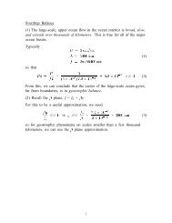
Turbulent diffusion….Simple advection-diffusion models can also beused to examine horizontal diffusive processes.Example: the 3 He plume in the S. Pacific

Turbulent diffusion….• • •• •••∂H∂H2U∂ x= κ xx2∂Lupton and Craig, 1981

Turbulent diffusion….Float dispersionshows thecharacter ofturbulence in thewestern N. Atlanticthermocline700 mThe plot shows the positions of 18 floats after one year.

Turbulent diffusion….Float dispersion atsub-thermoclinelevels of the N.Atlantic1300 m18 floats after one year, 1300 m

AuWiEddy kineticenergy by seasonat 900 m in thewestern N. Atlantic,inferred from floatdispersion.Sp[units: (cm/sec) 2 ]Suκ xκ y[units: 10 7 cm 2 /sec]

1000 mPacific float dispersion: anisotropic

[units: ergs/g][ (cm/sec) 2 ]Eddy kinetic energy in the Pacific

Atlantic•interior°•westernboundary°Pacific• ZONAL° MERIDIONALEddy diffusivity estimates scale roughly as EKE

Transient tracers and mixing….Tracers can beused with aknowledge oftheir sources andsinks todeterminecirculation andmixingThe history of CFC, 1930s - 2000

σ θ = 26.0Using the measuredvalues of CFC-11 andCFC-12, it is possibleto determine the ageof a water mass (ie,the time since it leftthe sea surface) andto infer pathways andstrengths of mixingand circulation.σ θ = 26.4[from Warner et al., 1996]

Oxygen in the ocean….Dissolved oxygen has a ubiquitous minimum at mid-depthin the world ocean….why?

Diffusion of dissolved oxygen….biological consumptiondCdt=2 2 2∂ C ∂ C ∂ Cκ + κ + κ + Rz ( )x 2 y 2 z∂x ∂y ∂z2Note that the minimum at mid-depth occursnearly everywhere. If we average the oxygendiffusion equation over the entire global ocean,and assume a steady state, we findw∂C∂ z=2Cκ ∂ + Rz ( )z∂z2O 2 : R(z) ∼ e αzRadioactive tracers:R(z) = −λC

Boundary conditions: C=C 1 at z=z 1 ; C=C 2 at z=z 2 ….[ Note: R(z) = R o e αz typically ]a typical solution