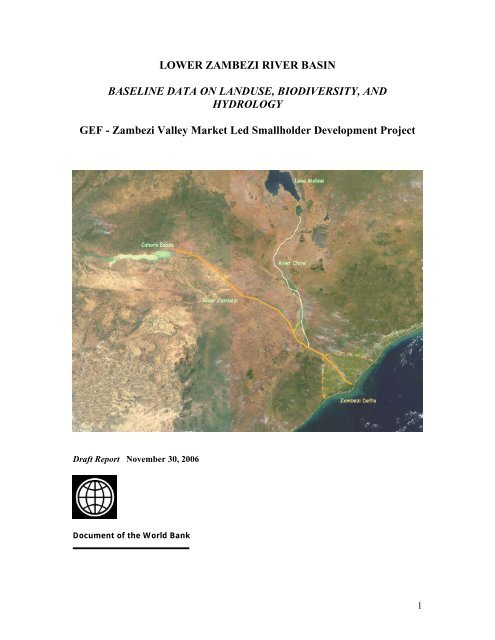
LOWER ZAMBEZI RIVER BASIN BASELINE DATA ON LANDUSE ...

LOWER ZAMBEZI RIVER BASINBASELINE DATA ON LANDUSE, BIODIVERSITY, ANDHYDROLOGYGEF - Zambezi Valley Market Led Smallholder Development ProjectDraft Report November 30, 2006Document of the World Bank1

ABBREVIATIONS AND TERMS________________________________________________________________________CBDCCDCENACARTADCBDIVERSITASDNADNGADPCAGISGOMGPSGPZIIAMLAIMICOAMODISNAPANBUNDVINEMPPFTSADCSPASRTMUEMUNFCCCVICConvention on Biological DiversityConvention to Combat DesertificationCentro Nacional de Cartografia e TeledetecçãoDepartment of Biological Sciences (Departamento de CiênciasBiológicas, Faculdade de Ciências (FC), Universidade EduardoMondlane (UEM)International Programme in Biodiversity ScienceNational Directorate of Water Affairs (Direcção Nacional deÁguas)National Directorate of Environmental ManagementProvincial Directorate for Environment (Direcção Provincial deCoordenação Ambiental)Geographic Information SystemGovernment of MozambiqueGlobal Positioning SystemZambezi Basin Development Authority of Mozambique (Gabinetedo Plano de Desenvolvimento da Região do Zambeze )Mozambique Institute for Agricultural Research (Instituto deInvestigacão Agraria de Mozambique)Leaf Area IndexMinistry for the Coordination of Environmental Affairs (Ministério paraa Coordenação da Acção Ambiental)Moderate Resolution Imaging SpectroradiometerNational Adaptation Programmes of ActionNational Biodiversity Unit (MICOA)Normalised Difference Vegetation IndexNational Environmental Management Plan (MICOA)Plant Functional TypeSouthern African Development CommunityStrategic Priority of AdaptationShuttle Radar Topography MissionEduardo Mondlane University (Universidade Eduardo Mondlane)United Nations Framework Convention on Climate ChangeVariable Infiltration Capacity (macroscale hydrologic model)________________________________________________________________________2

TABLE OF CONTENTSLIST OF FIGURES AND TABLES 4ACKNOWLEDGEMENTS 5EXECUTIVE SUMMARY 61. INTRODUCTION 91.1. Project Purpose 91.2. Background Information 91.3. Goal and Objectives 101.4. Scope of Work 102. LAND COVER AND LAND USE CHANGES VIA REMOTE SENSING 112.1. Background 112.2. Evaluation of Existing Remote Sensing and Map Data 122.3. A Comparative Estimate of the Land Use and Land Cover Changes 123. BIODIVERSITY ASSESSMENT 153.1. Background 153.2. Existing Biodiversity Information 153.3. A Rapid Appraisal Method 193.4 Indicators of Biodiversity and Potential Agricultural Productivity 213.5. Work Required to Deliver an Aboveground Biodiversity Baseline 233.6. The Status Quo of Biodiversity Baseline Information 243.7. Potential Coupling Biodiversity Data with Remotely Sensed and Hydrological Data 253.8. Biodiversity Survey and Global Benefits 284. THE DYNAMIC HYDROLOGY ANALYSIS FRAMEWORK 294.1. Background 294.2. Derivation of the Zambezi Valley River Networks/ Flow Accumulation Grid 294.3. Soils: From Type to Depth and Texture 314.4. Vegetation Classifications and Assumed Biophysical Attributes 324.5. Development of Climate Data 334.6. Evaluation of the Daily and Monthly Time Series of the Climate Variables 344.7. Evaluation of the Annual and Seasonal Climatology 364.8. River Discharge Data and Reservoir Operations 374.9. Generation-1 Vic Model Of the Zambezi 384.10. Training of GPZ and AraZambezi Staff 404.11. Zambezi Dynamic Information Framework (ZambeziDIF) Version 1 405. NEXT STEPS 425.1. Additional Needs For Remote Sensing Data 425.2. Biodiversity 425.3. Hydrology Modeling and ZambeziDIF 42REFERENCES 44ANNEX 473

LIST OF FIGURES AND TABLESFig. 2.1. Landsat spectral mixture analysisFig. 2.2. Numerical decision treeFig. 2.3. Land-cover MapFig. 3.1. Terrestrial ecoregion classificationsFig. 3.2. Layout of reference transects along the gradsectFig. 3.3. Plant species diversity and PFT diversity along the gradsectFig. 3.4. Course participants undertaking field training near MaputoFig. 3.5. DOMAIN potential mapping of the entire Zambezi basinFig. 3.6. Section of full Landsat scene showing results of a DOMAINFig. 3.7. Linear relationshipsFig. 4.1. SRTM-derived 3” (90-m) DEM of the Zambezi basin,Fig. 4.2. Routing network derived from the SRTMand Hydro1k basin delineationFig. 4.3. Soil properties across the Zambezi basin, of soil layer 1Fig. 4.4. Soil types of Tete, Sofala, and Manica provinces, at 1:1MFig. 4.5. WMO stations in and around the Zambezi basinFig. 4.6 ERA40 and WMO observed daily precipitation valuesFig. 4.7. ERA40 and WMO stations datasets monthly precipitationFig. 4.8. Daily maximum temperatureFig. 4.9. Monthly maximum temperatureFig. 4.10. Daily minimum temperatureFig 4.11. Monthly minimum temperatureFig. 4.12 Daily wind fieldsFig. 4.13 Monthly wind fieldsFig. 4.14. February 2000 daily average precipitationFig. 4.15. February 2001 daily average precipitationFig. 4.16. 1997-August 2002 daily average precipitationFig. 4.17. Gauging network of DNAFig. 4.18. Flows into and out of the Cahora Bassa reservoirFig 4.19. Flow regime at selected Zambezi stationsFig. 4.20. Modeled mean monthly discharge at Matundo-CaisFig. 4.21. Monthly average time series 1997-2006 of hydrologic variablesFig. 4.22 1997-August 2002 annual daily runoff averageFig. 4.23. 1997-August 2002 annual daily evaporation averageFig. 4.24. 1997-August 2002 annual daily soil moisture averageFig. 4 25. Schematic of prototype Zambezi Dynamic Information FrameworkTable 3.1 Comparative conservation status of biodiversity in MozambiqueTable 3.2 User-friendly indicator setsTable 3.3 Potential applications for different indicator setsTable 4.1. Relation of landcover schemesTable 4.2 Grid cells which have a stationTable 4.3 Characteristics of the Cahora Bassa dam.4

ACKNOWLEDGEMENTSThis report was prepared by Andrew Gillison (Vegetation Biodiversity), Gregory Asner(Land Use Land Cover Change), Jeffrey Richey (Hydrological Framework) and ErickFernandes (Land Management Advisor, ARD, World Bank). In depth technical assistancewas provided by Nathalie Voisin (lead, VIC), Lauren McGeoch, Harvey Greenberg, andDaniel Victoria. The studies would not have been possible without the active participation ofMrs. Samira Izidine, IIAM, Botany Department & National Herbarium, Mr. M.R. Marques,IIAM (soil inventory), Dr. João Cesar Santos and GPZ staff in Tete (Dr. Virgilio Ferrao),Quelimane (Mr. B. Gruveta) and Marromeu (Prof. P. Silva), Department of Agriculture staffin Maputo (Mr. Alvez) and Morrumbala (Mr. Moussa). Mr. Dinis Juizo (Eduardo MondlaneUniversity), and Mr. Jose Chembeze (AraZambezi and World Bank).The study team benefited greatly from collaboration and the support of World Bank staff inMaputo. We are grateful to Michael Baxter (Country Director), Daniel Sousa (Co-TTL),Eduardo Luis Souza (Cluster Leader), and Gregor Binkert (Lead Specialist) for theirguidance and logistics support. Mr. Daniel Sousa (Project Co-TTL) guided the field surveysand Mrs. Luisa Matshine provided invaluable travel and logistics support. Ms. K. Pangueneassisted with translation during the Biodiversity training course.5

EXECUTIVE SUMMARY1. Landuse/Landcover Change from Landsat. Remote sensing produced a multi-scaleanalysis of vegetation distributions:(1) For the study region, several images are available in data archives. Of the availableNASA ASTER, MODIS and Landsat 5 and 7 imagery spanning the period 1986-2005only three Landsat images met our criteria for science-quality data.(2) An initial analysis of March 1991 and December 2000 Landsat imagery showed thatperceived differences are far more sensitive to plant life cycle state than to land-coverchange. The floodplain region of the western portion of the Landsat images showedradical changes in both amount of flooded lands and the actual shape of the riverthroughout the region.(3) Examinations of Landsat imagery using composite analytical techniques, indicatedmapped areas of probable woodland/dense savanna, open savanna, herbaceousdominated,and degraded ecosystems.(4) The study has resulted in new and significant baseline knowledge about land cover in theproject area. It provides a live, spatially-referenced database for the Government ofMozambique (GOM).(5) Further analyses of land-cover, elevation and soil (topo-edaphic) conditions,climatological stress and plant life cycles (phenology) are needed and would require acombination of satellite data. The Zambezi Valley and surrounding region are dominatedby ecosystems displaying variation in vegetation structure and high seasonality.Therefore, it is important to discriminate between actual changes in land-cover (e.g.woodland clearing events) and plant phenological state. Further work should combinethe occasional high-resolution Landsat imagery with high-temporal resolution MODISimages to attempt a separation of phenology from land-cover changes.2. Biodiversity., Field survey and institutional information were used to assess biodiversitycoupled with capacity building:(1) Institutional information about biodiversity in the project area is poor to almost nonexistent.(2) An intensive training course on methods of rapid, aboveground biodiversity assessment(‘Training the trainers’) was completed for 13 participants (GOM, UEM) four of whomwere subsequently engaged in a biophysical baseline survey of the project area.(3) A survey of the project area was conducted using gradient-based (gradsect) methodologycovering key environmental gradients within the lower Zambezi valley. A standardprotocol was used to collect data that facilitates comparison with similar data collected inother countries. Additional data included soils and soil infiltration (for hydrology model)and landuse history.(4) Even allowing for a dry season, the baseline study reveals low levels of biodiversity whencompared to 27 other, mostly tropical countries. The low counts are offset by theoccurrence of numerous species of high horticultural significance as well as a number ofrare, endangered or vulnerable species.(5) Spatial data analysis using high resolution satellite imaging coupled with potentialmapping procedures indicates transects from the gradient-based survey represent morethan 90% of land cover variability in the lower Zambezi basin.(6) Detailed soil analyses and herbarium identifications are expected to reveal a closerelationship between plant-based biodiversity, aboveground carbon and potentialagricultural productivity. Preliminary analyses suggest simple, readily observable, plantbasedvariables can be used to indicate biodiversity that is relevant to land management,land use zoning and economic planning.6

(7) Baseline data (vegetation structure, plant species and plant functional types, includingadaptive photosynthetic attributes) can be quantitatively compared with remotely-sensed,biophysical variables. Initial findings reveal statistically significant relationships betweencombined sets of remotely sensed, photosynthetic, non-photosynthetic plant variables andsoil, and ground-based vegetation structure. As land cover varies with surface drainagepatterns, a close coupling is expected between the recorded plant and soil-based data,remotely sensed imagery and hydrological parameters.(8) Costing and logistic guidelines are indicated for future surveys.(9) The study highlights the global benefits of uniform survey technology to facilitatecomparison with other countries (e.g. biodiversity values, aboveground carbon) and tohelp evaluate tradeoffs between biodiversity management and income generation. Dataacquired along land use intensity gradients provide a framework for forecastingenvironmental change impacts on biodiversity and thus adaptive management options forSPA and related NAPA planning.(10) The study has resulted in new and significant baseline knowledge about biodiversity inthe project area. It provides a live, spatially-referenced database for the GOM and animproved operational framework and enhanced institutional capacity for the regionalassessment of biological diversity.3. Water Resources and Physical Data. A state-of-the art hydrology model and accompanyingdataset were used to derive:(1) A multi-scaled, high resolution, digital elevation model (DEM) capable of representingthe basic structure of the Zambezi basin, has established the central organizing constructfor the multiple information layers of the Baseline study.(2) Using the base DEM, elevation bands and a routing network file for river and flowaccumulation were derived for the entire Zambezi basin.(3) An evaluation of climate data was limited due to a data gap arising from the prolongedconflicts in Mozambique. Hence the convergence of two independent data streams wereevaluated: data records from the World Meteorological Organization (WMO), and thedaily re-analysis product (ERA40), from the European Center for Medium Range WeatherForecast (ECMWF). Despite some discrepancies between the ERA40 and the WMOstations datasets, it was possible to compile a useful database comprising daily andmonthly time series of the climate variables at specific grid cells and annual and seasonalclimatology.(4) The river flow regime of the lower Zambezi valley is dominated by the inputs to anddischarge from the Cahora Bassa dam. The overall flow regime reflects the pronouncedwet/dry season cycle while flow at Tete reflects the input of tributaries, including theRevubo river.(5) Detailed biophysical attributes of landcover for the Zambezi basin have been derived from1-km MODIS/TERRA products for the hydrology modeling and detailed Landsat analyseswere used to define the Smallholders target region. Soils (type, depth, texture) arerepresented at several scales, and for several sets of attributes with a three-layered depthprofile already partly calibrated.(6) The hydrology of the Zambezi basin is being simulated by the Variable InfiltrationCapacity Hydrology Model (VIC). Two VIC runs have been performed, one forced withthe 1994-2005 WMO stations datasets, and one forced with 1994-August 2002 ERA40datasets. A preliminary study shows that a minimum of 3 years of model initiation(spinup) is needed over the Zambezi Basin for the soil moisture to reach equilibrium.(7) Activities addressing data acquisition and modelling approaches for regional staff havebeen initiated, primarily with Eduardo Mondlane University (UEM) and Regional WaterAgency for the Zambezi (AraZambezi).7

(8) The data assembled for the land cover, biodiversity, climate, landuse and soils has beenassembled in a digital information framework (ZambeziDIF), which when combined withthe VIC hydrology model, will provide a potentially powerful analytical capability forallowing a range of stakeholders to examine current and future landscape and hydrologicaldynamics of the lower Zambezi Basin.8

1. INTRODUCTION1.1. PROJECT PURPOSE1. The Government of Mozambique (GOM) has requested the Bank to address the developmentconstraints and to improve small holder productivity by adopting a community demand-drivenapproach. The objective of the proposed Zambezi Valley Market Led Smallholder DevelopmentProject is to increase incomes of five selected districts through broad-based and sustainableagricultural growth. The Project will start operations in the two adjacent districts: Mutarara, TeteProvince and Morrumbala, Zambezia Province. Further three districts are proposed for inclusionduring the second year of implementation. Preliminary selection of the remaining three districtshas identified Mopeia in Zambezia province and Maringue and Chemba in Sofala Province,although these could be modified during the initial stage of implementation.2. The purpose of this study is to strengthen the capacity of the Ministry for the Coordination ofEnvironment Affairs (MICOA) to implement the Global Environment Facility (GEF)-financedcomponent of the Zambezi Valley Market Led Smallholder Development project and to collectquantitative baseline data that will facilitate an objective evaluation of the status of land coverand land use change dynamics over the last 10 years prior to the start of the Zambezi ValleyMarket Led Smallholder Development project.1.2. BACKGROUND INFORMATION3. The development objective of the Project is to increase the incomes of smallholderfarmers in selected districts of the Zambezi Valley region of central Mozambique. The GlobalEnvironment Objective is to limit and reverse land degradation and to improve ecosystemresilience towards climate change. The Global Environment Objective is also synergistic with thecreation of local benefits and improved livelihoods. Besides the national economic and socialbenefits of increased agricultural growth, the blending of the project with a Global EnvironmentalFacility (GEF) grant will significantly harness the potential synergies between national goals andglobal benefits such as reduced deforestation and the resultant global biodiversity loss andreduced greenhouse gas emissions while maintaining the functional integrity of both upland forestand lowland riparian ecosystems. For example, the current use of extensive farming methods isleading to increasing deforestation, land degradation, and further clearing of native woodlands asfarmers abandon degraded land. The loss of ecosystem services (local hydrology, habitats fornative biodiversity) from deforestation and land degradation is increasing the vulnerability oflocal communities to droughts and floods and markets.4. The project’s activities will directly address the negative environmental impactsidentified above and strengthen local and national capacity to integrate climate change risk intosustainable land management planning via the testing and calibration of dynamic vegetation, soil,hydrology model for improved predictive capacity of local climate change impact scenarios.Priority areas for improving land management to enhance adaptation include gallery forests andriparian zones which help to stabilize hydrological flows and thus reduce the possibility ofdegradation of existing agricultural lands. The resulting ‘avoided deforestation and reducedcarbon emissions’ are highly desirable outputs from an adaptation perspective.5. Key outcome indicators reflecting achievement of the Project development objective will be:the creation of social, physical and investment capital as well as associated market and supportsystems. The achievement of the global environment objective will be measured by: i) an increaseof at least 20,000 ha under improved SLM or natural resource management practices in Projectarea by Project end; ii) a measurable increase in biodiversity or carbon sequestration in targetedProject sites vs. control sites as measured by one or more of the following: (a) reappearance ofnative species, (b) increased carbon stocks, (c) reduced soil erosion, (d) reduced incidences of9

wild fires; iii) at least 3 predictive and basin specific hydrology-land cover-climate changescenarios for land use-land cover change impacts on hydrology under changing rainfall andevapotranspiration regimes; and (iv) increased use of drought-tolerant crops, fodder species andvarieties, crop rotations to increase soil organic matter, reduce weeds, and conserve soil moistureby local land users.6. Progress in achieving environmental targets will be measured by remote sensing and fieldsurveys in Project and control areas. An initial baseline beneficiary survey of almost 1,000 georeferencedhouseholds, which will include control areas, will be completed prior to Projecteffectiveness. A second impact evaluation survey will be carried out prior to the mid-term reviewand a final impact survey prior to the completion of the Project. Similarly, remote sensing withappropriate ground truth surveys and a GIS system will be used to establish the baselines for thenational agricultural and natural resource and the global environment indicators and outcomes.The Project will maintain both internal and external monitoring systems and conduct mid-termand end of the Project evaluations.1.3. GOAL AND OBJECTIVES7. The project goal is to enhance MICOA’s capacity to implement national environmentalprograms and to collect, safeguard, and provide effective web-based access to project data.8. The key objectives of the study are to:(1) Undertake a reconnaissance survey of land cover and land use types, aboveground plantbiodiversity, and hydrology resources in the five project districts and, if resources permit,extend data coverage over the entire the Zambezi valley (the Cahora Bassa lake to theZambezi Delta).(2) Use the reconnaissance survey to assess the adequacy, quality, and access rights ofexisting data sets.(3) Acquire additional remote sensing, land cover, biodiversity, and hydrology data via fieldcampaigns(4) Use data acquisition and evaluation events to train MICOA and Eduardo Mondlanestudents for future data acquisition campaigns.(5) Advise MICOA on the development of a web-based portal for data access bystakeholders.1.4. SCOPE OF WORK9. The study results in three distinct but related and geo-referenced outputs, summarized viaa dynamic information system:(1) Land Cover and Land Use Classes: A characterization of land use and land coverdynamics over the period 1995-2006 in at least the 5 project districts.(2) Vegetation Biodiversity: Provision of a geo-referenced plant biodiversity profile for the 5project districts, with rapid appraisal methods using low-cost, high-return, gradientdirectedtransects (gradsects).(3) A Dynamic Hydrology Analysis Framework: Deployment of geospatially-explicit,process based hydrology models that compute the water and energy balance of a spatialunit of the landscape (a “pixel”), as a function of landscape structure (topography, soils)and vegetation properties. Results from the individual project areas are combined into adynamic (indicating ranges of use) and flexible information system, the ZambeziDynamic Information Framework (ZambeziDIF).10

2. LAND COVER AND LAND USE CHANGES VIA REMOTESENSING2.1. BACKGROUND10. The primary reason for using remote sensing is to obtain total geographic coverage of aparticular set of environmental measurements of interest. The spatial coverage can range from asmall watershed or cropping system to the global environment. This type of wall-to-wallinformation cannot be readily acquired via field surveys or census data (but can be used to furtherinterpret and extrapolate outcomes from ground-based surveys). However, what remote sensingcan provide depends upon the geographic location and extent of the required information. Therequirements for geographic coverage thus directly impact the types of remote sensing systemsemployed and thus the type of information products that can be delivered. A closely related issueis that of temporal coverage: one must first determine if maps are needed on a weekly, annual oron-demand basis. In addition, the spatial resolution of the maps – household level, individualcrop fields, or continental-scale forests – must be determined. And most importantly, specificrequirements for environmental information must be defined. The intersection of theserequirements dictates the type and cost of the remote sensing measurements.11. Arguably the most important information provided by remote sensing is that of land-coverchange. Examples include the conversion of forests to managed grazing lands, the transformationof natural ecosystems to the built environment, and drainage of wetlands for croplands. Satellitesand aircraft can be used to monitor land-cover change, - the former usually more appropriate forworldwide use and repeat analysis. There are several satellites in low Earth orbit that provideremote sensing data for mapping land cover. These satellites differ in spatial resolution (andhence the smallest parcel of land that can be mapped), spectral resolution (hence the accuracy ofthe mapping), and temporal resolution (how often the mapping can take place).12. Although land-cover mapping is a key deliverable from satellite imaging systems, manyother ecosystem properties are critically important to land and aquatic management, conservationand policy development. Changes in ecosystem conditions and disturbance are some of the mostimportant issues requiring remote sensing vantage points. Drought stress, fire susceptibility, fireoccurrence, disturbance, and ecosystem degradation are examples of areas of significant researchand application in the remote sensing arena.13. In addition to the cost of acquiring satellite imagery, the cost of image analysis, mapproduction and validation are often unclear or unavailable to end-users. Many of the analyticalmethods are manual, and thus require significant investments to achieve large-scale mapping.The larger the area, the more expensive the manual approaches. In the case of land-covermapping, digital software analysis packages have been designed to help process imagery andprepare it for map production. The actual methods vary widely and are under constantdevelopment. Analysis of a single Landsat image covering 185 x 185 km can take a few months;analyses of multiple images can take much longer. A few new automated analytical methodshave been developed in the academic and private sectors.14. Global forest and deforestation monitoring systems are past the prototyping stage, and areproducing results that can be acquired via collaboration between users or the internet. Thesesources provide deforestation information for clearings of about 15-20 ha and larger, therebyfailing to detect the ubiquitous small land-holder clearings and forest disturbances (e.g., logging)that can dominate the forests of the world. To address this problem, several automated systems,have been developed very recently by private agencies.15. The type and accuracy of the mapping products derived for a custom-designed remotesensing project depends on the instrumentation used (e.g., data availability) and the algorithms11

employed. The image data most appropriate for a given project may or may not be available, andthis will have the largest impact on product development. From both instrumentation andalgorithm perspectives, a hierarchy of factors limits the delivery of a requested product. Forexample, a land cover map of forests, pastures, and croplands can be easily obtained from highspatial and spectral resolution imagery. However, similar types of land-cover mapping becomemore difficult as the spatial resolution decreases and the geographic cover increases. Analyses ofecosystem disturbance or conditions, such as drought stress or fire fuel load, have more compleximaging and analysis requirements. Therefore, specific types of imaging systems and analyticaltools are needed, thus increasing the cost of such projects.2.2 EVALUATION OF EXISTING REMOTE SENSING AND MAP DATA ON LANDCOVER AND LAND USES OF THE ZAMBEZI VALLEY16. Landsat imagery is ideal for monitoring a region such as the Zambezi Valley because theimages are of good radiometric quality and the spatial resolution of 30 x 30 m is excellent forland-cover analyses. We searched all relevant national and international data archives for Landsat5 and 7 imagery spanning the period 1986-2005. For the study region, there were several imagesavailable in these data archives, but only three images met our criteria for science-quality data.The criteria included: (1) nearly cloud-free imagery and (2) imagery unmanipulated prior toanalysis, thereby preserving the scientific integrity of the data. All other images were eithercloudy or had been sub-setted by collaborating agencies to the point at which the data could notbe reliably analyzed.17. Other imagery collections such as from the NASA ASTER and MODIS satellite instrumentswere checked for availability. Only the MODIS imagery was available on a regular basis since2000, but the spatial resolution of the land-cover products and spectral data is 1 x 1 km. Thisprecludes its use in the analysis of land-cover change in a region such as the Zambezi, wheremost changes occur at small grain size (

Asner et al. (2003, 2004) collected these spectral data using full optical range fieldspectroradiometers (Analytical Spectral Devices, Inc., Boulder, CO, USA). The spectralendmember database encompasses the common variation in materials found throughout forest,woodland, savanna, shrubland and grassland ecosystems, with statistical variability well definedand deemed viable for endmember bundling. The bare substrate spectra have been collectedacross a diverse range of soil types, surface organic matter levels, and moisture conditions.Spectral collections for NPV have included surface litter, senescent grasslands, deforestationresidues (slash), and other dry-carbon constituents from a wide range of species anddecomposition stages.20. With this method, the raw Landsat data are geo-corrected, then sensor gains and offsets areused to convert from digital number (DN) to exo-atmospheric radiance. The radiance data arepassed to the 6S atmospheric radiative transfer model (Vermote et al. 1997). A series of masksare designed to exclude clouds, water bodies, cloud shadows and non-image areas from theanalysis. Clouds are masked using the thermal channel (band 6) from the raw Landsat images.Water bodies are masked by finding pixels in the calibrated Landsat reflectance data containingbands 1 to 4 (blue to near-infrared). Cloud shadows are masked using an empirically-derivedcombination of the Landsat ETM+ reflectance values and the root mean squared (RMS) errorcalculations derived during the spectral mixture analysis. Rescaling of the mixture analysisresults is necessary to equalize very small (< 5%) differences in fractional cover results that occurdue to image calibration errors, residual atmospheric constituents (e.g., cirrus clouds and lightsmoke), and other random artifacts in the processing. This step produces a contiguous data setthat could then be readily analyzed for land-cover and vegetation conditions.21. In this preliminary study, we located Landsat imagery for the years 1991, 1999 and 2000.The 1999 and 2000 images were collected on August 22 and December 30, respectively. In thisimage pair, observed differences in vegetation properties were primarily caused by changes inplant phenological state. Changes in land-cover appeared minimal. An initial analysis of theMarch 1991 and December 2000 image also showed that perceived differences are far moreFig. 2.1 Landsat spectral mixture analysis, for images from March 1991, August 22 1999, andDecember 30, 2000. Whole image (upper images), with red rectangle indicating “zoom-in” for each.(lower images)13

sensitive to plant life cycle state than to land-cover change. In addition, the floodplain region ofthe western portion of the Landsat images showed radical changes in both amount of floodedlands and the actual shape of the river itself.22. The spectral mixture analysis described above provided quantitative data on land surfaceproperties within each 30m x 30m Landsat pixel covering more than 32,000 km 2 of landscapeeach year (Fig. 2.1). The results were 7-band images, where the bands are PV (photosyntheticvegetation), NPV (non-photosyntheticvegetation), bare substrate, standard deviation inPV, standard deviation in NPV, standarddeviation in bare, and root mean squared errorof the estimate. For each 30m x 30m pixel ineach image, these values were provided apercentage cover.23. The spectral mixture analysis results werethen classified into probable land-cover classesusing a numerical decision tree (Fig. 2.2). Theresulting maps indicated areas of probablewoodland/dense savanna, open savanna,herbaceous-dominated, and degradedecosystems (Fig 2.3).Fig. 2.2 Numerical decision tree used to classifybiophysical data into land-cover typesFig 2.3 Land-cover Map, 1991 (left) and 2000 (right). Green = woodland/dense savanna; Yellow =savanna; Blue = herbaceous-dominated; Red = degraded or disturbed14

3. BIODIVERSITY ASSESSMENT3.1. BACKGROUND24. Managing biodiversity at landscape level requires an adequate knowledge of the distributionof key elements of the biota and their environmental determinants including managementactivities. Traditional species-based, inventory methods are time-consuming, costly and in mostcases inappropriate for rapid evaluation or for monitoring purposes, particularly in developingcountries where institutional resources are limiting and where environments are frequentlycomplex and highly dynamic. The trend towards measuring both species and functional(adaptive) features of both plants and animals is gaining wider acceptance. Recent GEF-basedstudies in Brazil (Mato Grosso) involving intensive multi-taxon baseline surveys showed thatrobust, readily observable, plant-based biodiversity indicators could be derived for bioregionalplanning purposes. When matched with soil variables these indicators also revealed potentiallinks with agricultural productivity, thus providing a valuable knowledge base for enablingmanagement trade-offs for adaptive resource use. Parallel studies in Sumatra, Indonesia show thatreadily observable generic biodiversity indicators exist for lowland pantropical regions withsimilar environmental gradients and land use practices.25. Designing and implementing biodiversity baseline studies can be extremely costly and timedemandingif applied using standard statistical approaches and species-based inventory. For mostpurposes, rapid appraisal methods using low-cost, high-return, gradient-directed transects orgradsects are far more cost-effective. Gradsects are now widely used in surveys where there is aneed for rapid appraisal of the distribution of existing biota. They are now the preferred option forthe National Vegetation Classification of the mainland USA as implemented by the Parks Serviceand The Nature Conservancy. When coupled with a standard recording protocol (VegClass) forspecies, plant functional types (PFTs), vegetation structure and key site physical variables,gradsects provide an extremely useful means of rapidly establishing a knowledge baseline forplanning and management. The VegClass system is user-friendly and has been used in 12developing countries to successfully train personnel with limited field experience and for whomEnglish is not a first language. Unlike the majority of surveys that employ non-standardapproaches, data acquired from more than 1600 sites worldwide using the rapid survey VegClassprotocol provide a ready means of data comparison and evaluation.26. Biodiversity baseline data are but one element of the resource management matrix and aretoo often considered as stand-alone data. The reasons for this isolation from other data lie in thenature of the data that are often highly qualitative or else are restricted to species lists. To counterthis problem, the VegClass system includes rapid, quantitative measurements of plant featuresthat reflect plant adaptation to environment as well as vegetation structure, plant species and keysite physical variables. To be considered as a useful resource component, biodiversity should playan integral part in contributing to management goals in a way that facilitates decision-making andtrade-offs.3.2. EXISTING BIODIVERSITY INFORMATION FOR THE MOZAMBIQUEPORTION OF THE ZAMBEZI BASIN AND THE FIVE PROJECT DISTRICTS27. Living organisms – and hence biodiversity 1 are distributed mainly along deterministic,environmental gradients and rarely in a completely random pattern. For this reason theassessment of biodiversity in any one location must consider as far as possible, encompassing1 Defined as the variety of life on earth, usually expressed in terms of gene, species and ecosystem. Here weinclude functional (adpative) features of organisms as an integral component of biodiversity.15

iophysical gradients that influence the distribution and performance of both species andfunctional types 2 . Many plant and animal species in the project area for example, also occur inother regions of Southern Africa 3 . In reviewing the available biodiversity information of the twofocal districts of Mutarara and Morrumbala and the associated districts of Chemba, Maringue andMopeia, it is therefore necessary to consider the wider biophysical and geopolitical context ofMozambique and Southern Africa.28. Much of Mozambique’s biodiversity, particularly overall habitat quality, is recognisedinternationally and is arguably among the best preserved in Africa 4 (Table 3.1). This is due to acombination of relatively low demographic density, the general depopulation of rural areas over20 years of civil strife, and the underdeveloped basic infrastructure. In 1994 Mozambiqueestablished a National Biodiversity Unit (NBU) within MICOA, whose mission is to oversee theimplementation of the Biodiversity Convention in Mozambique. In 1996 the Government ofMozambique approved the National Environmental Management Programme (NEMP) thatrepresented the culmination of a series of initiatives and activities coordinated by MICOA.NEMP is the master-plan for the Environment in Mozambique. It contains a NationalEnvironment Policy, Environment Umbrella Legislation and an Environmental Strategy. One ofMICOA’s principal tasks in 1997 includedthe formulation and subsequentratification of a National Strategy andAction Plan for the Conservation ofBiological Diversity. Within theframework of this strategy, a number ofbiodiversity conservation issues are beingaddressed. These include technical, legal,political, cultural and socio-economicaspects of biological diversity. InsideMICOA, it is the National Directorate ofEnvironmental Management (DNGA),which deals with the three RioConventions (UNFCCC, CBD and CCD),and the DNGA has responsibility tocoordinate with other institutions theimplementation of these conventions 5 .Mozambique is also signatory to theSADC Regional Biodiversity Strategy 6that aims to provide a framework forregional cooperation in biodiversity issuesthat transcend national boundaries. Asmost biodiversity issues in SADC aretransnational, this is a logical developmentin biodiversity conservation. The SADCMember States are also signatories to theTable 3.1 Comparative conservation status ofbiodiversity in Mozambique2 Used here in the sense of adaptive features of individual organisms that contribute to dispersal andsurvival and that influence the way ecosystems respond to environmental change.3 Typically taxonomic elements of Mopane and Zambezian woodlands and forests that include members ofthe Mimosoideae (e.g. Acacia spp.) and Caesalpinoideae (Bauhinia, Colophospermum spp.)4 Centre for Environment Information & Knowledge in Africa (CEIKA)5 MICOA: Mozambique Initial National Communication to the UNFCCC. (2003).6 SADC (Southern African Development Community) consists of thirteen Member States: Angola,Botswana, the Democratic Republic of Congo, Lesotho, Malawi, Mauritius, Mozambique, Namibia, SouthAfrica, Swaziland, Tanzania, Zambia and Zimbabwe.16

CBD.29 The country of Mozambique (801,590 km 2 ) contains a wide diversity of terrestrial,freshwater and marine habitats. However, the biodiversity of Mozambique is poorly known andpoorly documented due to a number of factors including lack of human resources, lack ofopportunities to carry out field-studies during the period of civil unrest and weak institutionalcapacity. A limited amount of data is available for some taxonomic groups, but some pre-wardata especially those dealing with land cover are outdated. Existing knowledge is dispersed overvarious sectoral agencies as well as with individuals in the form of project documents, reports,scientific articles, maps, aerial photographs and satellite imagery. The information has not beenintegrated at the national, local and even in some cases the institutional level. In addition, datasets are based on different classification systems, organized along different formats and are ofvarying accuracy.30. A number of biodiversity mapping and inventory activities have been undertaken, or areunderway. But, as may be expected, in the absence of baseline data, there is little accurateinformation (with a few notable exceptions in National Parks and Game Reserves) regardingtrends in biodiversity and processes or activities threatening biodiversity.31. The five districts are located along the lower Zambezi valley that serves as a biodiversitycorridor from the uplands in Tete Province to the expansive 12,000km 2 Zambezi delta in SofalaProvince. While little is known of biodiversity within the five districts, considerable national andinternational interest focuses on the delta – one of the largest wetland systems in southern Africa.The Zambezi river basin, the largest basin entirely within the SADC region is rich in wetlands.The basin drains a total area of almost 1.4 million km 2 , and wetlands cover almost 66,000 km 2with a total water storage 7 estimated at 100,000 million m 3 . In 2003, the GOM declared theMarromeu Complex of the Zambezi Delta to be the first Wetland of International Importance inMozambique under the Ramsar Convention. The Ramsar Convention is the world’s foremostinternational agreement for the protection and wise use of wetlands, and requires nationalcommitment to the sustainable management of designated wetland sites. The complex is host tomany large mammals and birds 8 . While most conservation management tends to focus on fauna,much less activity is directed to documenting the flora - an exception being the relatively speciesrichGorongosa Reserve further.32. Water resources development projects have substantially altered the hydrological regime ofthe Zambezi Delta and impacted biodiversity 9 . Prior to the construction of Kariba Dam on themiddle Zambezi River, peak floods spread over a mosaic of vegetation communities. Floodplaingrasslands were inundated with floodwaters for up to nine months of the year, with many areasbeing saturated throughout the dry season. With the closure of Kariba Dam in 1959 and CahoraBassa Dam in 1974, nearly 90% of the Zambezi catchment has become regulated so that thenatural flood cycles of the lower Zambezi River cannot be maintained. Flooding events in thedelta, when they occur, now depend on local rainfall-runoff or unplanned (possibly catastrophic)water releases from the upstream dams. These hydrological changes are further exacerbated bythe construction of dikes along the lower Zambezi that prevent medium sized floods up to 13,000m 3/s from inundating the south bank floodplains. The implications for biodiversity in the face ofthese hydrological changes in the delta are profound and must be considered in the context of thehydrogeomorphic processes that control vegetation distribution and abundance. Woody savannaand thicket species have increased in density and colonized far into the floodplain grasslandmosaic. Relatively drought-tolerant grassland species have displaced flood-tolerant species in the7 http://www.sardc.net/imercsa/zambezi/Cep/fsheet16/index.htm8 The International Crane Foundationhttp://www.savingcranes.org/conservation/our_projects/program.cfm?id=239 Timberlake, J. (1998).17

oad alluvial floodplain, and saline grassland species have displaced freshwater species on thecoastal plain 10 . Reduced water levels are associated with the loss of some mangrove communitiesand increasing marine saline intrusion where salt-tolerant tree species (e.g. Acacia xanthophloia)are appearing for the first time 11 . According to local villagers at Luis on the north-eastern bank ofthe Zambezi river near Doa in the Mutarara district, changes in river levels have also led toalterations in riparian vegetation and land use pattern where Phragmites reed-dominated riparianswamps are a valuable natural resource 12 .33. Due partly to the paucity of baseline information in the five districts, vegetationclassification has developed onlyalong very broad lines 13 . Previousland use studies 14 covering certainsections of these districts dealtmainly with classifications aimedat serving agricultural rather thanecological or conservationinterests. However these in-depthstudies together with an intensiveecological study of the Gorongosareserve 15 , contain much valuableintegrated (plant, animal and soil)information that is yet to besystematically addressed. With theexception of some of thecomponent species, the vegetationand land cover patterns observed Fig. 3.1 Terrestrial ecoregion classifications [1] covering the areain the 1970’s differ significantly under study (ellipse with dashed lines). These include Mopanefrom the present-day and and Zambezian Woodlands (AT0725), Southern Miombosubsequent changes in the Woodlands (AT0719), Eastern Miombo Woodlands (AT0706),hydrodynamic systems of the Zambezian Coastal Flooded Savanna (AT0906), Southernlower Zambezi valley . These Zanzibar Woodlands (AT0128) and East African Mangrove(AT1402).earlier attempts at classificationhave been superceded by a more recent mapping of the world’s ecoregions 16 (Fig. 3.1).34. The six ecoregional types outlined in Fig 3.1 illustrate ecosystem variability within the lowerZambezi basin. The existing boundaries are nonetheless questionable given the broad,overlapping distribution patterns of many component species of each ecoregional type. Dominanttree species such as Mopane (Colophospermum mopane) and Brachystegia spp. are widelydistributed across vegetation formations broadly classified as Miombo, Mopane and Zambezianwoodlands where mapped boundaries have become further blurred due to recent, decadal changesin land use patterns and hydrological regimes (See also Annex Figs 3,4). In assessingbiodiversity within the five districts it is therefore necessary to regard such classifications asindicative at best and instead, focus on the key species and the environmental factors most closelyassociated with their present distribution.10 Beilfuss et al. (2001).11 P. da Silva GPZ, Marromeu (pers. com. 16 Sept. 2006)12 Thompson (1985)13 See White (1983)14 Loxton et al. (1975a,b)15 Tinley (1977)16 Olson and Dinerstein (1998), Olson et al. (2002)18

3.3 A RAPID APPRAISAL METHOD AND A STANDARD PROTOCOL FORQUANTITATIVELY ASSESSING VEGETATIVE BIODIVERSITY FOR THE ZAMBEZIVALLEY PROJECT SITES35. The aim of the baseline study is to provide both a relevant knowledge base for ongoingassessment of the GEF project 17 and a methodological framework for future informationgatheringas well as an opportunity to train a group of Mozambican specialists in survey designtechnology and field sampling procedures. A related aim is to establish a cost-effective, standardmodus operandi and enhanced institutional capacity for a more detailed study of the project areawhile keeping in mind other areas within Mozambique. It is important to that beyond these aimsit was not the intention of the field study to comprehensively document and analyze the entirefive districts and the surrounding region.36. In cases such as the present study where a key objective is to determine the distributionpattern of biota, purposive sampling along environmental gradients considered to be important ininfluencing the distribution of plants and animals, is likely to be more cost-effective thantraditional statistical sample designs employing random or purely systematic (e.g. grid-based)approaches. A theoretical and practical basis for such a methodology is embodied in gradientdirectedtransects or gradsects 18 where sample sites are located within a nested hierarchy ofdeterministic environmental variables. A typical hierarchy might range from climate (e.g. rainfallseasonality) gradients through geomorphology and primary, secondary and tertiary drainagepatterns and soil types down to natural and modified land cover and land management facets. Thegradsect approach is currently being used to classify and map the vegetation of the mainlandUSA 19 and is being increasingly adopted in a number of tropical countries. A comparativeevaluation in South Africa 20 showed that gradsect method out-performed other survey methodsinvolving both plants and animals. For the present project, the gradsect approach was appropriatefor the survey of plant species given the need to sample a range of nested environmental factors(rainfall seasonality, parent rock type, drainage patterns, land cover and land use types).37. In order to provide an environmental context for the project area, especially for the two focaldistricts of Mutarara and Morrumbala, a gradsect was established from Tete in the northwest tothe Chinde/ Nicoadala/ Marromeu districts near the Zambezi river delta. While the gradsectfollowed the general Zambezi valley drainage system it also accommodated a primary rainfallseasonality gradient and a sequential series of underlying geological formations and soil typesthat were further sampled according to variation in land cover and land management type (seeexamples in Annex Figs 3,4,5). The gradsect was designed using all available information fromGOM Ministries including IIAM 21 (herbarium and soils) DNA and CENACARTA 22 where mapsof geology, soils, administrative boundaries and topographic at 1:250,000 scale were obtained ineither hard copy or electronic format. Satellite imagery (Landsat) covering the lower Zambezivalley, was examined in conjunction with MODIS imagery and a digital elevation model (DEM)derived from shuttle radar (SRTM30) at 30m grid resolution (see Section 2. Land cover and landuse changes via remote sensing). Preliminary stream flow and runoff models derived from VIC (Section 4) also provided a basis for site selection. In July 2006 a four-day reconnaissance of theproposed gradsect was conducted by road prior to the main survey in which the team 23 gathered17 Zambezi Valley Market Led Smallholder Development Project18 Gillison and Brewer (1985).19 USGS-NPS (2003).20 Wessels et al. (1998).21 Instituto de Investigação Agraria de Mozambique.22 Centro Nacional de Cartografia e Teledetecção, Mozambique23 E.C. Fernandes (team leader), J. E. Richey (hydrologist), A.N. Gillison (biodiversity specialist).19

significant information on landcover and land use including plantbiodiversity composition andrichness in key vegetation types.This information together with thatobtained from local villagers andgovernment representativesprovided both hard data and areconnaissance overview that wereinvaluable in designing thesubsequent baseline survey. Thefinal survey was completed in tendays in September 2006 in whichthe placement of sample transects(Fig. 3.2) was completed withassistance from local landholderswho provided important informationabout site history and landmanagement practices. Teammembers 24 included a pedologist,forest ecologist, social geographerand field botanist all of whom hadcompleted a previous intensivetraining course in rapid biodiversityassessment conducted by the teamleader at Eduardo MondlaneUniversity in Maputo.Tete (Mphanda Nkuwa)MopeiaQuelimaneFig. 3.2 Layout of 32 (40x5m) reference transects (red dots)along the gradsect from Tete (Mphanda Nkuwa) to the deltaregion near Chinde. Blue indicates the lower Zambezi valleycatchment area as detected from Shuttle Radar Imagery (SRTM;Section 4). Black and white zones indicate areas outside theZambezi basin.38. In each transect the team used a standard recording protocol (VegClass 25 ) to collect aspecific set of biophysical data that included georeferenced (GPS) site physical variables as wellas all vascular plant species and plant functional types (PFTs) (Annex, Table 1.). The VegClassprotocol has been used to record such data from more than 1600 transects worldwide andprovides a quantitative basis for readily comparing data within and between regions. In additionto this protocol, soil samples were collected for laboratory analysis (IIAM, Maputo) andclassified in field according to the USDA Soil Taxonomy. Plants were identified by local as wellas scientific names where available and botanical voucher specimens were collected for eachspecies in each transect for later identification at the IIAM herbarium in Maputo. Because theoverall baseline study aims to integrate the biophysical field data with a hydrological model ofvariable infiltration capacity (VIC) of the lower Zambezi river basin, the team collected soilinfiltration data (Annex, Table 2) using a modified infiltrometer 26 for potential input to thismodel. At each transect, information on land use history was also recorded in discussion withland owners. This type of information will assist in describing land management types for theproject area and, when linked with the biodiversity information, is expected to play a key role indeveloping subsequent decision support systems for sustainable land use management.24 A.N. Gillison (team leader), J. Mafalacusser, (pedologist, IIAM), A. da Fonseca (geographer, GPZ), H.Pacate (forest ecologist, DPCA MICOA), A. Banze (field botanist, IIAM).25 Gillison (2002)26 A 110mm plastic pipe inserted 2 cm into ground into which 1 liter of water was poured and timed tocomplete infiltration (a ‘falling head’ infiltrometer). A mean was taken from two samples in each transect.20

39. Georeferenced, digitalphotographs were taken of landcover at each transect and acomplete set distributed to teammembers including personnelconcerned with processingremotely sensed imagery.40. The survey was completedduring the height of the dry season.The team estimated that not lessthan 80% of the landscape hadbeen fired between MphandaNkuwa in Tete Province and thedelta near Chinde (97 km southeastof Mopeia) (Annex Fig.3).These conditions made difficult thelocation of representative, nonfiredsites and also reduced thePlant species diversity50 Spp diversity = - 1.272 + 1.260 PFTsRSq (adj.) = 0.9804030201000 5 10 15 20 25 30 35Plant Functional Type diversityFigure 3.3 Plant species diversity and PFT diversity alongthe gradsect [29] . Transects indicated by red dotsnumber of plant species available for documentation. At the same time the team acquired criticalinformation about the state of vegetation during such an extreme period and was able to comparethe state of the same transects recorded during the previous reconnaissance. In 32 transects theteam recorded 183 unique PFTs and 192 (provisional) plant species. Due to extremes of theseasonal climate and recurrent fires, many species respond by reverting to more than one PFT (forexample, tree to multistemmed, rhizomatous shrub). The ratio of diversity of species to PFTs isexpected to decrease even further as harbarium identifications reduce the number of speciesthrough synonomy. Other transect data including vegetation structure, species, PFTs and sitephysical features are listed in Annex (Tables 3-7). The statistical relationship between plantspecies and PFT diversity 27 is unusually high (RSq (adj.) 0.980) (Fig 3.3) and reflects therelatively low number of species and species:PFT ratio recorded per transect. The graphindicates that where field identification of species is problematic, counts of readily observable,unique PFTs can be used instead to estimate species richness with a high degree of confidence.3.4. A SET OF VARIABLES FOR SUBSEQUENT TESTING WITHIN THE PROJECTDISTRICTS AS INDICATORS OF BOTH BIODIVERSITY AND POTENTIALAGRICULTURAL PRODUCTIVITY INCLUDING ABOVE-GROUND CARBON41. Intensive multi-taxa biodiversity baseline studies carried out in paleotropic Sumatra,Indonesia and neotropical Mato Grosso, Brazil 28 produced biodiversity indicators that could beused by persons with relatively little training. Where species identification is difficult, readilyobservable features such as PFTs or elements of vegetation structure can be used. Table 3.2. listsTable 3.2 User-friendly indicator sets for biodiversity, potential agricultural productivity andaboveground carbon (based on case studies using the VegClass system)Cover-BasalLitterCover-IndicatorPlantabundanceMean Canopy height (m) Area PFTDepthabundanceset(m 2 Specieswoody plts)(cm)bryophytes

variables under different groupings that might be applied might be applied for different purposesand different scales as outlined in Table 3.3.Table 3.3 Potential applications for different indicator setsIndicatorsetApplicationSensitivitySpatial mapping scaleA- rapid assessment and monitoring of ecosystem health- compatible with remote sensing- estimator of above-ground carbon- primary level planning and land use zoninglow1:250,000to1:1,000,000B- above, plus broad indicator of plant and animal habitat- indicator of ecosystem productivity- indicator of biodiversity- biodiversity and land use zoningmedium1:50,000to1:250,000C- above, plus higher level indicator of biodiversity- indicator of animal habitat- improved estimator of site productivity potential- fine scale mapping of biodiversity unitsmediumtohigh1:50,000D- above, plus fine scale indicator of specific animalhabitat- indicator of site productivity potentialhigh1:10,00042. In previous studies in tropical countries, all the variables listed above have shown highlysignificant correlations either with plant species diversity, aboveground carbon or diversity offaunal groups such as bird, mammals and termites 29 . Of these indicators litter depth is one of themost potentially useful indicators of animal habitat. However none of the regions surveyed inBrazil or Indonesia was subject to the seasonal extremes of the Mozambique survey area or to theannual regimes of man-made fire where most litter is destroyed. For this reason the predictivecapacity of plant litter in the lower Zambezi valley should be tested following the wet seasonwhen there has been sufficient litter build-up and when higher levels of plant and animal speciesdiversity are most likely to occur. Methodological details of how such variables are measured areoutlined elsewhere 30 .43. Together with the plant-based assessment, detailed soil analyses will add significantly to theGOM database on regional soil types. It is expected that when combined with the biodiversitydata, soil-plant relationships will provide a useful scientific basis for coupling biodiversityindicators with soil features and thus potential agricultural productivity. As yet it is not knownwhether soil infiltration data will provide an additional, useful parameter for VIC. However, theinfiltration data were generally consistent with soil texture associated with the soil taxonomicclasses as identified in the field. The use of VegClass structural data for estimating abovegroundcarbon in the project area remains to be validated. Access to existing models of carbondistribution for Africa 31 may prove useful in developing surrogate models for estimatingaboveground carbon in the five districts based on vegetation structure and remotely sensedimagery.44. An intensive training course was delivered at Eduardo Mondlane University in Maputo withthirteen participants. 32 Field exercises were completed over two days in a forest reserve on theoutskirts of Maputo (Fig. 3.4). Standard VegClass field books, and a CD-ROM containing29 Gillison et al (2003), Jones et al. (2003)30 The VegClass Training Manual. In: Gillison, A.N (2006)31 Brown and Gaston (1980) and Walker and Desanker (2004)32 (Annex I, Table 8)22

VegClass software and training manualtogether with the DOMAIN potentialmapping software was supplied to allparticipants. Despite dry seasonal conditionsin the field, participants performed well.Field data were collected by each participantindividually and participants werepartitioned into four ‘teams.’As part of thecourse procedure, the group data weresubsequently compiled and analysed in theclassroom where an evaluation highlighteddifferences in group performance. Thesedifferences were further analysed and led toimproved undertsanding of the methodologyby participants. On completion, anevaluation of the course was led by D.Sousa of the World Bank at a meeting thatFig. 3.4 Course participants undertaking field trainingnear Maputowas attended by all course participants as well as representatives of MICOA, IIAM and UEM. Ageneral consensus was that the course had been successful. Formal Certificates indicatingsuccessful completion of the course were awarded to all 13 participants.45. On completion of the course four participants (A. Banze, J. Mafalacusser, H. Pacate and A.da Fonseca) traveled to Tete for the field survey of the five districts. During that survey theparticipants received additional tuition and in the second half of the survey accepted theresponsibility of locating transects and recording and compiling field data. This additional fieldtraining enhanced their capacity to design and implement basic biodiversity surveys – a tasklikely to be easier during a wet rather than a dry season phase. Additional tasks such as samplingsoil and soil transmissivity (infiltration) added to the reality of an integrated baseline survey. Theteam performed very efficiently under unusually trying field conditions.46. At the completion of the survey a presentation of the preliminary survey results wasdelivered to previous course participants at the World Bank office in Maputo, with additionalattendees from MICOA and IIAM. Presenters, including some team members, outlined some ofthe difficulties associated with surveys implemented during the driest season and all were ingeneral agreement that, while the methodology could be satisfactorily applied during any season,end-of-wet-season surveys were like to prove the most cost-efficient. A conclusion of the survey– that the data reflected low biodiversity levels, was met with some disquiet by certain agencyrepresentatives (IIAM, MICOA) who felt that such information, if widely distributed, might bedetrimental to biodiversity conservation in the region. It was pointed out that, while other surveyswere yet to be completed, the team identified other significant features of biodiversity such asunique habitat and floristic elements and that these should offset any immediate concern.3.5. ADDITIONAL WORK REQUIRED TO DELIVER AN ABOVEGROUNDBIODIVERSITY BASELINE FOR THE PROJECT DISTRICTS47. Laboratory soil analyses and plant identifications from the present baseline survey areunderway at IIAM. The present survey provided sufficient information to facilitate the design andimplementation of a more detailed plant-based baseline survey of the five project districts. For thefollowing survey the following, mainly logistic, criteria should be taken into account:(1) Sample design and implementation should follow the same procedures that wereimplemented in the preliminary baseline survey. However additional (e.g. ethnobotanicaland land use history) information should be included in the survey protocol.23

(2) Survey should commence at the conclusion of the wet season when roads are accessible.(3) Mobility is essential. A single team of five personnel should undertake the survey (Teamleader and ecologist, botanist and assistant, soil specialist (e.g. pedologist) and socialscientist (geographer). A compact team of this size provides sufficient space in vehiclesto allow local landholders to acompany the team to survey sites.(4) Two 4wd vehicles plus drivers are needed to transport personnel and field samples.(5) Participation with local landholders is essential and requires their prior consultation.(6) The survey should be restricted to the five districts but the team leader should considerthe possible inclusion of associated areas in close proximity to the Zambezi river (e.g. thedistricts of Caia and Marromeu) to add value to the overall assessment of environmentalaspects.(7) Where possible the team should liaise closely with any agency involved in householdsurveys in the area as this will greatly enhance the prospects of developing an integratedknowledge base for planning and management purposes.(8) At least one team member should receive further training in data analysis includingspatial data analysis. Alternatively, a specialist in such procedures could be hired prior toand following the baseline survey.(9) Appropriate Ministeries and institutions and other stakeholders (e.g. socioeconomists andregional planners) should be advised before a baseline study is commenced and wherenecessary should be involved in the process of survey design.(10) Prior to survey, agreements should be reached with research and other institutions likelyto be concerned with soil analyses and curation of botanical material.48. Based on present findings it is envisaged that a single 5-member team could undertake adetailed biodiversity assessment of the five districts within a period of approximately four to sixweeks depending on field conditions. Costs in USD for certain items will depend on conditions atthe time of survey but should include:(1) Vehicle hire (e.g. GPZ Tete) and fuel.(2) Survey equipment: GPS ($350) , prismatic compass ($80), Bitterlich prism for basal areaestimation ($60), binoculars (8x40) ($120), secateurs x 2 ($50), digital camera (min 5Megapixels) $350. Topographic maps 1:250,000 scale ($100), Miscellaneous items($300). Total ca. $1410.(3) Airfare costs to and from Maputo to Tete (depending on location of personnel)(4) Airfreight costs to an from study area (equipment and samples) (approx. $800)(5) Accommodation: unknown. It is recommended that the team be accommodated underroof rather than undertake camping as the latter is not conducive to logistic efficiency.(6) Daily fees and/or per diems to be negotiated with respective individuals and theirinstitutions.(7) Institutional costs for soil analyses and botanical identification should commit analyticaland technical resources for a period of not less than five months.(8) Additional costs for the hire of a spatial data analyst ( two months immediately postsurveyand three months after completion of soil analyses and plant identification)(9) The acquisition of appropriate remotely sensed imagery should be considered prior tosurvey. Imagery acquired for the present baseline survey may be adequate for asubsequent survey of the five districts.3.6. THE STATUS QUO OF BIODIVERSITY BASELINE INFORMATION WITHINTHE PROJECT DISTRICTS OF THE ZAMBEZI BASIN49. As indicated above, biodiversity baseline information is institutionally poor to non-existent.This is consistent with the lack of available capacity and the historical background of inventoriesthat contained a largely agricultural or commercial bias. Historical and recent vegetation24

classifications within the region are of little value for management and are only broadly indicativeof biodiversity pattern for survey design purposes.50. Given the current paucity of data, the present survey has added significantly new baselineinformation to the GOM knowledge base. In ten days a highly mobile team of five specialistswith one week of prior intensive training in assessment methods was able to document keyfeatures of environmental gradients and patterns of biodiversity richness and composition acrossthree Provinces (Tete, Sofala, Zambezia) and eight districts (Cahora Bassa, Moatize, Mutarara,Morrumbala, Marromeu, Mopeia, Chinde and Nicoadala). The 32 transects deployed along thelower Zambezi gradsect provide an important environmental context for the future selection ofsample sites within the five districts. The baseline survey included all ecoregions in Fig. 2.1, inaddition to recording biodiversity in both relatively natural and intensively managed land usetypes including monocropping sequences in flooded riparian systems in Mutarara, slash and burnsubsistence gardens near Chinde and a commercial, irrigated plantation in Marromeu.51. In global terms the lower Zambezi valley subregion is low in biodiversity. Despite theeffects of the dry season and fired landscapes, this conclusion is generally consistent withfindings from other researchers in the Mopane- Brachystegia forests and woodlands. Datarecorded from the same transects in July and September revealed little change other thanincreased deciduousness. Reasons for low biodiversity are not clear but appear to be associatedwith generally low levels of labile soil nutrients that are likely to be continually removed fromthese ecosytems by annual firing. In Southern Africa low biodiversity is not necessarilyassociated with low biodiversity – the southern Cape Fynbos heaths on sandstones provide anexample of high biodiversity associated with low soil nutrients. In Mutarara skeletal soils onRhyolite rock outcrops (Transect 11 Chinsomba) also supported relatively high species and PFTdiversity.52. Criteria for biodiversity conservation should not be driven by high diversity alone but shouldinclude other criteria such as endemicity, plant functional diversity, uniqueness of habitat andvulnerablility. When these are considered, the lower Zambezi valley contains outstandingexamples of unique biodiversity features, especially among succulent (Euphorbiaceae,Agavaceae, Apocynaceae) and primitive (Zamiacaeae) genera. All are of significant interest tothe global horticultural and floricultural community and may be of economic potential if suitablemarkets could be established. While present findings are indicative of the basic status quo ofbiodiversity for this subregion, a more intensive survey will better quantify the biodiversityvalues of the project area.3.7. PROSPECTS FOR COUPLING BIODIVERSITY DATA WITH REMOTELYSENSED AND HYDROLOGICAL DATA FOR MODELLING PURPOSES53. Preliminary analyses indicate that biodiversity data acquired from this survey can beeffectively coupled with remotely sensed data. Land cover expressed as different classes ofvegetation (savanna, deciduous broadleaf forest, woodlands…) compiled for the Zambezi basinfrom global data 33 were overlaid by the 32 transects as a check for vegetation representativenesswithin the region. A potential mapping program DOMAIN 34 was used for this purpose and theresults (Fig. 3.5) show that the gradsect reflects the majority of vegetation types below 500melevation .33 N.Voisin and L McGeoch, Hydrology Group, Civil and Environmental Engineering, Univ. Washington,Seattle USA.34 Carpenter et al. (1993)25

54. The same exploratory mappingprocedure can be used to detectsimilarity patterns for specific featuresof biodiversity such as levels of plantfunctional or species richness, specificsets of species assemblages and,possibly aboveground carbon. Moredetailed biophysical values ofremotely sensed imagery that detectvarying levels of photosynthesis anddead or dying vegetation (e.g. asreflected in NDVI) have been assessedfor example in some African Miombowoodlands 35 . This type of imagerymay provide an interpretative linkwith PFTs that are described viaVegClass according to theirphotosynthetic envelope as well as lifeform.55. A complete Landsat scene 36covering the central portion of theproject area was used to generate datafor photosynthetically active, nonphotosyntheticallyactive and soil(bare ground) – components thattogether indicate a measure of landcover. These three data layers werecombined and analysed using theDOMAIN potential mapping programto generate an environmental envelopeor “domain” for 16 of the 32 surveytransects included in the central scene.This environmental domain was thencompared with the data values for theentire Landsat scene and similaritylevels mapped (Fig.3.6). The mapshows that better than 90% of landcover as represented by the compositesatellite imagery is accounted for bythe 16 transect locations. As furtherdata come to hand from herbariumidentifications and soil analyses ofthese transects, it will be possible toproduce spatially-referenced mapsindicating levels of selectivebiodiversity features for this section ofFig 3.5. DOMAIN potential mapping of the entire Zambezibasin with 32 survey transect points located lower leftwithin dotted line. Colors indicate similarity of anenvironmental envelope computed for the 32 points andcompared with land cover (percentage of vegetation classin each pixel for 8 key vegetation types within the basin).Red indicates similarity >95% grading through orange,yellow, green to blue that is < 5% (typically upland zones)Fig. 3.6. Section of full Landsat scene 167/72 (Dec 2000)showing results of a DOMAIN analysis of ‘Land Cover’ asindicated by composite photosynthetic and nonphotosyntheticvegetation and soil (bare ground) imagery. Of32 transects 16 (circular white dots) were included in the fullscene. When an environmental domain envelope generated for16 transects is compared with values for the entire scene,mapped similarity levels are indicated by color (red = >95%similarity grading downwards through orange --> yellow ->green to blue (

in addition, provide an important reference database and analytical framework that will enhanceinstitutional capacity for any subsequent regional biodiversity assessment.56. A preliminary analysis of composite sets ofsatellite and ground-based data revealssignificant underlying statistical relationshipsbetween ‘Land cover’ (expressed asphotosynthetic, non-photosynthetic and soil(bare ground)) and ground-based estimates ofvegetation structure (expressed as basal area ofall woody plants, mean canopy height and plantlitter depth) (Fig. 3.7). As more data come tohand, the derived satellite imagery is beingfurther explored for possible inter-linkagesbetween the different data areas (hydrology,biodiversity), for example, moisture gradients,soils and specific plant assemblages. Ifconfirmed, linkages of this kind will greatlyassist the development of an integratedanalytical framework for both the project areaand the wider area of the lower Zambezi basin.57. Specific examples of plant-based parametersin the hydrology model (VIC) that have possiblelinks to related PFTs and other VegClassvegetation structural attributes recorded in fieldinclude:Landsat 2000 Pv, Npv, Soil3210-1-2Satellite (Land cover) = -0.0000 + 0.7015 Ground Vegetation structure( P < 0.002, RSq (adj.) = 0.456 )-3-2.0 -1.5 -1.0 -0.5 0.0 0.5 1.0 1.5Basal area (m 2 ha -1 ), Mean canopy height (m), Litter depth (cm)Fig. 3.7 Linear relationship between Multi-Dimensional Scaling (MDS) of satelliteimagery (Land cover) and ground survey ofvegetation structure is highly significant.(P < 0.002) [ Pv = photosynthetic, Npv =non-photosynthetic, Soil = bare ground ].Transects (solid red circles) occur within oneLandsat scene of the central project area.• OverstoryIn VegClass defined by mean canopy height and further modified by percentage ofcanopy cover divided into woody and non-woody components.• Architectural resistanceUnknown – but possibly quantifiable through furcation index of woody canopy• Aerodynamic resistanceUnknown – but possibly quantifiable through furcation index of woody canopy• Minimum stomatal resistanceRelated to PFEs leaf size class, leaf inclination class, succulence and whether leavesare isobilateral or dorsiventral• Ratio of total tree height that is trunkAccessible through canopy profile sketch of transect and onsite digital photography• Monthly leaf area indexLAI is based on a laterally inclined dorsiventral leaf. As such LAI makes no directallowance for succulent, partially deciduous, or isobilateral leaves or leaves that areeither vertical or pendulous in inclination. Perhaps explore how LAI can be adjustedaccording to estimated percentages of these variables in each transect.• Monthly vegetation heightUnlikely to change significantly within 12 months for mature woody plants. InVegClass definable through mean canopy height.• Rooting depthNo field data for this variable that is extremely difficult to quantify. It may bepossible to base estimates on depth and texture of soil (recorded in the presentsurvey).27

Other survey data included soil infiltration rate and plant litter depth 37 . Informal observationssuggest plant litter depth may be a significant factor in run-off and is likely to vary with season inthe project area, especially given the high incidence of fire.3.8. BIODIVERSITY SURVEY AND GLOBAL BENEFITS58. International agencies such as the CBD and DIVERSITAS emphasize the need for uniformtechnology that can be used to collect data to facilitate comparison of biodiversity within andbetween regions. To date such technology has not been forthcoming. The present technologyaims to satisfy this need. To that end both the gradsect survey methdology and the VegClassrecording system have been evaluated in more than 1600 sites worldwide. This procedure hasfaciltated detailed comparison and analysis between a number of countries and regions. Anexample of how global data might be compared is illustrated in Annex , Table 9 where at thesimplest level, plant-based diversity is compared for the richest forest sites recorded in 28different countries including Mozambique. Annex Fig. 1 illustrates comparative differencesbetween countries when plant species diversity is regressed against PFT diversity along gradientsthat reflect land use intensity as well as naturally-occuring vegetation. Again, the overalldiversity levels for Mozambique are consistent with other general reviews of the vegetation types(e.g. Mopane woodland) that cover much of the project area.59. As indicated above, field estimation of aboveground carbon and carbon sequestration,although highly desirable for global benefits, can be problematical. In the Miombo WoodlandsRegion of south-central Africa, it is estimated that 50–80% of the total system’s carbon stock isfound in the top 1.5 m belowground and that this decreases markedly under agricultural land use38 . Soils from a wide range of land use types obtained in the present survey will be examined fororganic carbon and these values related to aboveground vegetation structure and PFTs. Shouldthe relationships prove to be statistically significant as in previous studies (e.g. Sumatra 39 ) thenadditional analyses will be undertaken to explore such correlates on further surveys in the projectarea. Together with estimates of aboveground carbon based on allometric studies of vegetationstructure in similar landscapes elsewhere, these results may contribute to indicator potential at abroader global level.60. The data acquired from the present survey of land use types can help derive an empiricalmodel of how biodiversity is likely to vary along a land use intensity gradient. This type ofinformation is potential useful where there is a need to help forecast the impact of environmentalchange on both biodiversity and related agricultural productivity and to assist with decisionmakingfor adaptive management. The approach is consistent with SPA and the aims and goalsof the National Adaptation Programs of Action (NAPA) in Mozambique as approved by the GEFin 2002.37 Annex I, Tables 2 and 6 respectively38 Walker and Desanker39 Gillison (2002a)28

4. THE DYNAMIC HYDROLOGY ANALYSIS FRAMEWORK4.1. BACKGROUND61. The overall goal of the modelling approach is to facilitate the development of climate changeand land cover-land use change scenarios to provide responses to the following kinds ofquestions:• What would be the impacts of changes in agriculture (including irrigation) and forestrypractices on local and regional water balances? E.g., will re-forestation lead to an increaseor to a decrease in streamflow?• How would changes in landuse practices, with varying climate, affect water supply andwater quality?• If some indication of climate over a growing season was provided, could crop selection (andfire management) be improved?• Can floods or droughts be predicated, or at least anticipated, one or two months into thefuture, as an early-warning system? These models compute not only stream discharge, butsuch intermediate products as soil moisture and evapotranspiration. If a model is maintainedin an operational mode, the current conditions of soil moisture (the antecedent for floods ordrought) can be monitored. If the hydrology modelled is then driven by forecasts fromregional climate models (see below), then near-future potential conditions can be tracked,and warnings given.• How would developments of infrastructure affect downstream flow, water quality, andfisheries resources?• How would changes in streamflow affect fisheries (including through changes in waterlevels of nursery areas)?62. Multiple, complex data “layers” are required to address these questions, and to analyze thepast, current, and future dynamics of the target Districts, in the context of the overall Zambezibasin. The inter-relation of the information described above, with the additional informationrequired to describe water movement requires a sophisticated structure to process the information.Hence a “Zambezi Dynamic Information Framework” (ZambeziDIF) is being developed thatincorporates (a) a physical template module (describing static properties of topography and soils),(b) a land use/ land cover module (describing not only what is present, but the biophysicalattributes of the vegetation), (c) a surface climate module (providing the drivers for the landsurface model, and (d) a geospatial landscape/hydrology model. By virtue of its data requirementsand its outputs, the hydrology model provides the construct for the overall ZambeziDIF.63. Different landscape/hydrology models are typically required for different scales. For example,a distributed model such as the Distributed Hydrology Soil Vegetation Model (DHSVM) could bedeveloped for the project districts over which digital topographic data allows explicitrepresentation of surface and subsurface flows with landcover changes, at 150-m resolution (eg.Rattanaviwatpong et al in press). But given data scarcity and the requirements to place the targetdistricts in the context of the overall basin, the Variable Infiltration Capacity (VIC) model, asemi-distributed macro-scale hydrologic model, which represents explicitly the effects ofvegetation, topography, and soils on the exchange of moisture and energy between the land andatmosphere (Liang et al., 1994; Nijssen et al., 1997, 2001b) is used here (described in moredetail, Section 4.7).4.2. DERIVATION OF THE ZAMBEZI VALLEY RIVER NETWORKS/ FLOWACCUMULATION GRID USING BEST AVAILABLE SRTM DATA29

64. A multi-scaled digital elevation model (DEM) capable of representing the basic structure ofthe Zambezi basin, from the entire basin to “zooming in” at high resolution for the individualSmall Holders districts, establishes the central organizing construct for the multiple informationlayers of the Baseline study. To serve as the topographic base data model for the overallSmallholders project, a DEM (Fig. 4.1) was derived from the CGIAR version of the 3” (90-m)Version 2 (finished) SRTM DEM. Each 3" cell is the mean of the component 1" cells. The DEMwas processed by:(1) placing a no-data area in the alluvial fan of the Cuanda River,(2) filling all sinks in the DEM,(3) computing flow direction,(4) calculating the watershed grid,(5) calculating the contributing area (in square km) for each grid cell, and(6) calculating the cubic km of water falling upstream of each cell (based on 1995rainfall).Shaded relief was calculated is a simple derivative of the DEM. The base DEM was enhancedwith waterbodies from the SWBD dataset derived from the 1" SRTM data by NASA, and withpolitical boundaries and, lakes, and rivers are extracted from VMAP0.Fig. 4.1 SRTM-derived 3” (90-m) DEM of the Zambezi basin, with progressive “zoom-ins” from wholebasin to Smallholder districts65. The VIC hydrology model requiresproducts derived from the base DEM.(1) Elevation Bands. Instead of assuminga constant and smoothed precipitation rateover the entire grid cell, VIC useselevation bands in order to vary theprecipitation rate and type over differentfraction areas of the grid cell. Thisprovides better snow estimation, althoughthis is not essential over the ZambeziBasin. That is why only five elevationbands were derived.(2) Routing Network File. The directionfiles for the routing network (Fig. 4.2)were derived from the SRTM30 version 2DEM and the Hydro1k basin delineation,Fig. 4.2. Routing network derived from the SRTM30 andHydro1k basin delineation. For subsequent model analysis,the stations at Zumbo (1), Revuboe (2), Tete (3), MatundoCais (4), Megaza (Chire, 5), and Luenha (6) are indicated.30

using mostly ArcInfo spatial analyst functions (fillsink, flowacc). A in-house program equivalentto “flowdir” was used to determine the direction file in the format used by the routing model.Several significant lakes (area larger than a 90m grid cell) are present in the basin, in particularCabora-Bassa, Kariba, Malawi, Chilwa and McIlwaine. The soil characteristics for LakesMalawi, Cahora-Bassa and Kariba could not be derived and limited a VIC run on this area.Similarly, the routing direction file is not sufficiently accurate in this area. A different approachusing the newer VIC version dealing with lakes will be necessary for those specific cells.4.3. SOILS: FROM TYPE TO DEPTH AND TEXTURE66. Soils are represented at several scales, and for several sets of attributes. For the purpose ofthe hydrologic modeling, a basin-wide soil file is used as a mask file and also specifies soilcharacteristics of each grid cell (Fig. 4.3 The soil column is being divided into three layers. Thefirst layer is arbitrarily set to 10 cm. The second and third layer depths will be calibrated and are,arbitrarily, presently set to set to 50 cm and 250cm deep. Bulk density, and sand and claycomponents were derived through the SoilProgram (Carter and Scholes, 2000) for each grid cell.Information comes from the World Inventory of Soil Emission Potentials (WISE) pedon database (Batjes, 1995). Other required soil characteristics were derived from a look up table (Cosby1984), which specifies porosity, hydraulic conductivity, field capacity and wilting point based onthe soil texture ( related to the sand and clay components).Fig. 4.3 Soil properties across the Zambezi basin, of soil layer 1.67. For higher resolution purposes in the Small Holder districts, a 1:1 million map by soil typesand their attributes is available, through IIAM. (Figure. 4.4)Fig. 4.4 Soil types of Tete, Sofala, and Manica provinces, at 1:1M (IIAM)31

4.4. VEGETATION CLASSIFICATIONS AND ASSUMED BIOPHYSICALATTRIBUTES68. VIC requires two land cover inputs: the vegetation parameter file and the vegetation libraryfile. The vegetation parameter file describes the land cover composition and rooting depthdistribution of each VIC grid cell. The vegetation library file is a look-up table that details variousphysical attributes (e.g. trunk ratio, albedo, surface roughness, etc.) of each land cover type. Moreinformation about the required land cover inputs for VIC can be found athttp://www.hydro.washington.edu/Lettenmaier/Models/VIC/Documentation/Documentation.html. The basis for a vegetation parameter file for the Zambezi watershed was the MODIS 12Q1dataset, entitled “MODIS/Terra Land Cover Type Yearly L3 Global 1km SIN Grid.”Documentation and metadata for this dataset are available athttp://lpdaac.usgs.gov/modis/mod12q1v4.asp. The MODIS 12Q1 dataset includes severaldifferent classification schemes; the Type 1 (IGBP) classification, which divides the land surfaceinto 17 different land cover types, was used here. Some scan-related classification error in certainparts of the watershed was detected in the down-loaded data. Although the 0.05 degree productseemed to contain little scan error, the 1km dataset contained important detail that would be lostif the lower resolution product was used.69. There were approximately 100 land cover pixels (1km resolution) contained within eachVIC grid cell (1/12 degree resolution). To determine the land cover composition of each VIC gridcell, ArcMap 9 was used to derive the percent cover of each IGBP land cover type within eachVIC grid cell. Less than 1% of the land cover pixels within the watershed were unclassified. Todeal with unclassified pixels, the percent cover of each land cover type in a VIC grid cell wasdivided by the percent cover of all classified pixels in the VIC grid cell. This approach effectivelyconverted the unclassified pixels in each grid cell to different land cover types based on thecomposition of land cover types within the grid cell. Each land cover type was also assigned to aspecific distribution throughout the three soil layers. There are 4 types of root distributionavailable: uniform (same amount of roots in each soil layer), linear increase (fraction of rootsincrease with depth), linear decrease(fraction of roots decreases with depth)and triangular shape (most of the rootsare in the middle soil layer).70. To develop a vegetation libraryfile for the Zambezi basin, the globalvegetation parameter set developed byLDAS (Land Data AssimilationSchemes) was used. Documentationand metadata for this parameter set canbe found online athttp://ldas.gsfc.nasa.gov/LDAS8th/MAPPED.VEG/LDASmapveg.shtml. Theclassification scheme used to developthe LDAS parameter set was notidentical to the IGBP scheme. The twoclassification schemes are related asoutlined in Table 4.1. Since there is nopermanent snow or ice in the Zambezibasin, any pixels classified by MODISas “permanent snow and ice” wereassumed to be misclassified byTable 4.1. Relation of landcover schemesIGBP classLDAS parameters classWaterWaterEvergreen needleleaf forest Evergreen needleleaf forestEvergreen broadleaf forest Evergreen broadleaf forestDeciduous needleleaf forest Deciduous needleleaf forestDeciduous broadleaf forest Deciduous broadleaf forestMixed forestsMixed CoverClosed shrublandsClosed shrublandOpen shrublandsOpen shrublandWoody savannasWoodlandSavannasWooded GrasslandGrasslandsGrasslandPermanent wetlandsCroplandsCroplandUrban and built-upUrban and built-upCropland/natural forestmosaicPermanent snow and ice Bare ground(misclassification error)Barren or sparsely vegetated Bare ground32

MODIS’ automated classification procedure. There were only about 260 such pixels in thewatershed. These pixels were assigned the same vegetation parameters as the “bare ground” landcover class. To obtain parameters for IGBP classes that had no comparable class in the LDASclassification, the appropriate LDAS classes were combined.71. The monthly data in the LDAS parameter set follow a northern temperate seasonal cycle,where leaf coverage is highest around June-July and lowest around December-January. In orderto more accurately represent deciduous seasonality in the Zambezi basin, all of the monthlyparameters from LDAS were inverted so that values for June became values for December,values for July became values for January, and so on. Some of the parameters required for theVIC vegetation library had no appropriate counterparts in the LDAS parameter set. Where therewere no appropriate LDAS data, default data from the sample VIC vegetation library (online(online at ftp://ftp.hydro.washington.edu/pub/HYDRO/models/VIC/Veg/veg_lib) were used.4.5. DEVELOPMENT OF CLIMATE DATA72. Climate data constitute one of the most important, and the most problematic, data sets forevaluation of the Zambezi basin. Coverage and coordination of data from individualmeteorological observation stations across the 8 nations of the Zambezi valley is not trivial. Ofparticular concern is the data gap due to the prolonged conflicts in Mozambique. Hence a strategyof evaluating the convergence of two independent data streams: data records from the WorldMeteorological Organization (WMO), and the daily re-analysis product (ERA40), from theEuropean Center for Medium Range Weather Forecast (ECMWF) was adapted.73. 134 WMO stations datasets with observations in the 01/01/1994-12/31/2005 period wereretrieved. Fig. 4.5 shows the location of the stations and the fraction of the record that is missingover the 1994-2005 period. Those stations observations (precipitation, maximum and minimumtemperature and wind) have been regridded using an inverse square distance interpolation (Symapalgorithm; Shepard 1984) into the 17208 grid cells included in the Zambezi Basin mask at 1/12 thof a degree resolution. Only valid observations are used for this regridding. Temperature fieldshave been corrected with a constant lapse rate of -0.065 (degree per meter) in order to adjust thetemperature at thestation altitude to thegrid cell meanelevation. Theregridding has beendone using a minimumof 4 stations and amaximum of 80stations. Missingrecords are still presentafter the regriddingwhen the 80 neareststations have missingdata. There are 54 dayswithoutanyobservations over the134 stations in theoriginal and thereforealso the regriddedWMO datasets.Fig. 4.5. WMO stations in and around the Zambezi basin, with the numberof missing daily observations in the 1994-2005 period (4383 days)33

Persistence was used to assign precipitation on the days where data were still missing afterregridding. In particular, as ERA40 and WMO stations datasets period do not overlap, ERA40values could not be substituted. One should also note that most of the WMO stations with littlemissing observations are located south of the Zambezi Basin, which can have an impact inrepresenting the spatial distribution of precipitation during extreme events (February 2000 and2001 for example). See comments on that later.74. While the ERA40 product provides a 40-year record, the 1979-08/2002 period is the mostconsistent period in terms of technology of observations. ERA40 provides a global dataset ofmeteorological variables (accumulated precipitation, average air temperature and zonal andmeridional wind components) on a N80 Gaussian grid (1.125 degree resolution at the Equator)and at a 6 hourly time step. The maximum (minimum) temperature has been assigned themaximum (minimum) 6 hourly temperature average for simplicity. The 6 hourly precipitationdata has been accumulated to a daily time step and the wind speed has been derived from the 6hourly wind components and then averaged over the day. The dataset has then been regriddedusing the same algorithm explained earlier, to the 1/12 th of a degree resolution, and using aminimum of 4 and a maximum of 12 nearest grid cells in the original grid.75. The ERA40 griddeddataset is then compared tothe WMO station griddeddataset for the accumulatedprecipitation, minimum andmaximum temperature andwind for the 1994-08/2002period. The comparison ismade in two parts. The firstpart compares the dailyvariables at grid cells wherestations are located in thebasin and have less than 1000missing records even afterregridding (see earliercomment). 11 WMO stationscorrespond to this criterion as shown on Table 4.2.Table 4.2 WMO stations located in the Zambezi Basin , that haveless than 100 missing record ( over 4383 record, i.e. about 23%)Station Name Country Lat Lon missingrecordsKasane BC -17.81 25.15 520Lusaka (Mil/Civ) ZB -15.31 28.45 737Bulawayo/Woodvale ZW -20.01 28.61 527Gokwe ZW -18.21 28.93 930Gweru/Thornhill ZW -19.45 29.85 638Harare/Kutsaga(Mil) ZW -17.91 31.13 522Kariba ZW -16.51 28.88 743Karoi ZW -16.83 29.61 772Mount Darwin ZW -16.78 31.58 981Mutoko ZW -17.41 32.21 769Victoria Falls ZW -18.1 25.85 9394.6. EVALUATION OF THE DAILY AND MONTHLY TIME SERIES OF THECLIMATE VARIABLES AT SPECIFIC GRID CELLS76. Fig. 4.6 shows the daily at the 11 grid cells including the 11 WMO stations (Table 4.2)mentioned earlier. A few very large values (larger than 200mm a day) have been reported and donot correspond to any large values in nearby days in the other 10 grid cells (11/26/98, 336mmm;12/27/96, 306mm; and 12/15/95, 205mm). ERA40 and WMO stations daily precipitationdatasets do not agree well. Fig. 4.7 shows the comparison of monthly WMO stations and ERA40datasets. Part of the differences can be explained by the missing WMO stations data replaced bythe values of the previous non missing day value. But significant differences remain.77. Figures 4.8 and 4.9 show the daily and monthly maximum temperatures, and figures 4.10and 4.11 the minimum temperatures. As expected, the comparison shows better results than withprecipitation. The ERA40 maximum temperatures are very close to the WMO stations dataset andthe minimum temperatures are consistently higher (due to the fact that the minimum 6 hourly34

ERAERAWMO StationsFig. 4.6 ERA40 and WMO observed dailyprecipitation values (mm) over the 1994-08/2002 period in 11 grid cells.WMO StationsFig. 4.7 ERA40 and WMO stationsdatasets monthly precipitation (mm) forthe 11 grid cells.average ERA40 temperature are compared with real daily minimum temperatures observed by theWMO stations). Maximum temperatures seem to be less sensitive. Maximum and minimumtemperatures are used to derive solar radiation in the VIC hydrological model. The hydrology isless sensitive to this uncertainty in solar radiation, due to the bias in the minimum temperature,than to the differences in precipitation between the two datasets. Figures 4.12 and 4.13 show thewind field. Both the daily and monthly wind comparisons show a reasonable agreement: ERA40wind usually overestimates WMO stations wind for low wind values.ERAERAWMO StationsFig. 4.8 Daily maximum temperatureWMO StationsFig. 4.9 Monthly maximum temperatureERAERAWMO StationsFig. 4.10 Daily minimum temperatureWMO StationsFig 4.11 Monthly minimum temperature35

ERA40WMOFig. 4.12 Daily wind fields (m/s)WMOFig. 4.13 Monthly wind fields4.7. EVALUATION OF THE ANNUAL AND SEASONAL CLIMATOLOGY78. The temperatures and wind comparison at the 11 grid cells for the WMO stations andERA40 are comparable. However there is a disagreement in the precipitation that might bepartly due to the fact that most all the stations with less than 10% (and even 50%) of missingobservations are in the southern part of the basin. Fig. 4.14 shows the lack of localizedprecipitation pattern over the 1997-August 2002 climatology. Especially in case of extremeevents like the floods in South Mozambique (Limpopo) in February 2000 (Fig. 4.15) causedby extreme rainfalls in the Limpopo basin (and south of the Zambezi basin), and theZambezi floods in February 2001 (Figure 4.16) due to intense rainfall in the central part ofthe basin is better represented in ERA40.Fig. 4.14 February 2000daily average precipitation(mm/day)Fig. 4.15 February 2001daily average precipitation(mm/day)Fig. 4.16 1997-August 2002daily average precipitation(mm/d)36

4.8. RIVER DISCHARGE DATA AND RESERVOIR OPERATIONS79. The stage height (relative depth) and discharge of the Zambezi River and its tributaries is theresponsibility of the Direcçãcao Nacional de Águas and AraZambezi, through measurementsacross a gauging network (Fig. 4.17). Rating curves (the process for translating stage todischarge) are sparse, and available data records are being parsed together.Fig. 4.17 Gauging network of DNA (base topography)map form DINAGECS, O.J. Sibia, 2005).80. The flow regime of the lower Zambezi valley is dominated by the inputs to and dischargefrom the Cahora Bassa dam Table 4.3, Fig. 4.18). The overall flow regime reflects thepronounced wet/dry season cycle, as discussed above (Fig. 4.19). Flow at Tete does reflect theinput of tributaries, including the Revubo.Table 4.3 Characteristics of the Cahora Basa dam.Catchment Area (km 2 ) 1,239,800Flow 10,000 year frequency 28,000(m 3 /s)ReservoirVolume available/Total (km 3 ) 52/65Volume available/Total (GWh) 13000/16500Submerged Area (km 2 ) 2660Length (km) 270Width max (km) 30Discharge (m 3 /s)1500012000900060003000Inflow (by mass balance)OutflowDam- double curvature archMax height above foundation 164(m)Max width at foundation (m) 21.5Crest Level/length (m) 331/303Total discharge capacity 139390Oct’00 Oct’01 Oct’02 Oct’03 Oct’04 Oct’05 Oct’06Fig. 4.18 Flows into and out of the Cahora Bassareservoir, Oct 2000-Sep 200637

600TeteCBRevuboDischarge (m 3 /s)Mainstem Stage (m)E-320 TeteE-293 MutararaE-291E-285 Marromeu10E-288E-302E-104Tributary Stage (m)E-348E-646E-64540020064864212 24 36 48 60 72212 24 36 48 60 7212 24 36 48 60 72Days (from Oct 1 2004)Fig 4.19 Flow regime at selected Zambezi stations: (left panel) discharge at Cahora Bassa, Tete andthe Revubo (by Tete), (middle panel) stage height at mainstem stations, (right panel) stage at majortributary stations.4.9. GENERATION-1 VIC MODEL OF THE ZAMBEZI81. The hydrology of the Zambezi basin is being simulated by the Variable Infiltration CapacityHydrology Model (VIC) developed at the University of Washington and Princeton University. InVIC, the subsurface is characterized in the vertical direction by three soil layers. The top soillayer contributes to runoff via fast response mechanisms (“quickflow”), and the deepest soil layerproduces base flow. Drainage between the soil layers is modeled as gravity driven. Controls ofvegetation on evapo-transpiration are represented explicitly using a Penman-Monteithformulation, while baseflow is represented as a non-linear recession. Sub-grid variations inprecipitation rate and temperature, due to variations in elevation, are represented by sub-dividingeach grid cell into a number of elevation bands. Daily precipitation, maximum and minimumtemperature, and wind speed are the primary meteorological variables that drive the model.Downward solar and longwave radiation, and dew point temperature, also used to force themodel, are derived using algorithms that relate them to either the daily temperature, thetemperature range, or both (Maurer et al., 2002). The model used to simulate the routing ofstreamflow along the stream network (Lohmann et al., 1996, 1998) uses a triangular unithydrograph and linearized St. Venant’s equations to route the streamflow from each individualgrid cell separately to the basin outlet through the channel network. The routing model does notexplicitly account for channel losses, extractions, diversions, or reservoir operations, but coupledsub-models can account for these flow modifications (e.g, Costa-Cabral et al.in review). VIChas been applied to all river basins in the U.S. (Abdulla et al., 1996; Cherkauer and Lettenmaier,1999; Maurer et al., 2002; and Nijssen et al., 1997); the entire country of China (Su and Xie,2003); and the Mekong Basin (Costa-Cabral et al a,b, in review). VIC is set up here to run at adaily time step at both 0.5 degree and 1/12 th of a degree spatial resolution over the Zambezi Basin82. Application of VIC requires the development of a set of input data files, includingmeteorological forcing (land surface climatology of daily precipitation, minimum and maximumtemperature, and winds), vegetation attributes by vegetation class, a river network derived from adigital elevation model, and river discharge history at select stations. The data sets described inthe previous Tasks were set up and incorporated into the VIC model structure. The initialapplication of VIC modelled the flow regime at Matundo Cais, for the period 1980-August 2002,38

PrecipitationRunoffEvapotranspirationSoil MoistureFig. 4.20 VIC-modeled (0.5 o resolution) monthly meandischarge (m3/s) at Matundo-Cais, 1980-2003, withERA40 climatologyFig. 4.21. Monthly average time series 1997-2006 of precipitation and simulatedhydrologic variables (R, ET, SM; in mm)with a simulation of 0.5-degrees (Fig. 4.20). Two VIC runs were then performed, one forced withthe 1994-2005 WMO stations datasets, and one forced with 1994-August 2002 ERA40 datasets(Fig. 4.21-4.24). Only 1997-August 2002 or 2005 are presented next as 3 years were allowed forspin-up (model initialization). A preliminary study (not shown) showed that a minimum of 3years of spin-up was needed over the Zambezi Basin for the soil moisture to reach equilibrium.Fig. 4.22 1997-August2002 annual average dailyrunoff (mm)Fig. 4.23 1997-August 2002annual average dailyevaporation (mm)Fig. 4.24 1997-August 2002annual average daily soilmoisture (mm)83. These results, while preliminary and uncalibrated, show that the dynamic model can capturethe basic dynamics of the overall basin. Precipitation can not only be computed, but translated torunoff. As part of this process, the “internal’ dynamics of the hydrologic cycle are computed,including soil moisture and evapotranspiration. The ability to explicitly trace spoil moisture is39

critical to the assessment of water availability for agriculture, under different landuse and climatescenarios.4.10. TRAINING OF GPZ AND ARA ZAMBEZI STAFF ON THE DATAACQUISITION AND MODELLING APPROACHES84. Activities addressing data acquisition and modelling approaches for regional staff wereinitiated, primarily with Dinis Juizo (Eduardo Mondlane University) and Jose Chemba(AraZambezi, now World Bank). Mr. Juizo has been active in data acquisition, and has begunthe process of downloading the VIC model code.4.11. ZAMBEZI DYNAMIC INFORMATION FRAMEWORK (ZambeziDIF)85. The database and models that are being developed in the ZambeziDIF in support of thisSLM baseline study are extensive, and represent information not previously available inMozambique. Much of the information is represented as geospatial data layers, in ArcGIS rasterformat (which can be converted to other geospatial formats, including GridASCII suitable for awide range of industry standard GIS applications). To facilitate initial access to this information,the ZambeziDIF represents constructed data layers through ArcIMS (Arc Internet Map Server).The user does not need to have specialized GIS or visualization software available. ArcIMSessentially provides a user with access to the data layers; including being able to query andexamine the data, as if the user has GIS software.86. ZambeziDIF Version 1 can be accessed at:http://www.riversystems.washington.edu/zambezi_dif (it is expected to migrate to hosts inMozambique at the earliest opportunity). Categories of information include (Fig. 4.24):Physical templateZambezi Basin Boundaries: Basin boundary (the mask of the Zambezi basin), politicalboundaries, lakes and rivers (from several sources), DEM derived from SRTM, and a series ofLandsat tiles for 1990 and 2000 (as composites only; not processed)Soil Properties: The hydrologic properties required by VIC, including soil density, bulk density,Ksat, DSmax and PCP.Vegetation and LanduseSouthern Africa MODIS Landcover: MODIS-derived land cover products at 1km and 8 km forSouthern Africa, as the overall coverage of the regionLandcover and Landuse: MODIS 1-km landcover, and the Landsat TM5 and ETM productsdescribed in Section 2.VIC Landcover 8 km: The percent landcover in each pixel, for each of the classes (cropland,savanna, etc) utilized by VIC, derived from the MODIS 1 km data.Surface Climate Inputs and Model-Computed Hydrology (based on the ECMWF ERA-40 data):This set includes the surface climate forcing variables required by VIC (temperature,precipitation, wind) and model output products (runoff, evaporation, and soil moisture). Timeperiods include the mean annual over the period 1997-2002, and February 2000 and 2001.40

Southern Africa MODISZambezi BasinVIC LandcoverSoilLandcover and LanduseSurface Climate and Model-Computed HydrologyFig. 4.25. Zambezi DIF Version 1. The composite geospatial information used in the overall baselineis represented in a set of 6 ArcIMS (internet map server) projects, accessible athttp://www.riversystems.washington.edu/zambezi_dif). Clicking on a data layer will access it (withoutthe user needing GIS software), and allow data queries.87. The ZambeziDIF, combined with the VIC hydrology model, will contain a potentiallypowerful analytical capability for allowing a range of stakeholders to examine current and futurelandscape and hydrological dynamics of the lower Zambezi Basin. For example, the draft reportfor Sustainable Water Resources Development for Irrigated Agriculture calls for exactly such acapability.41

5. NEXT STEPS5.1. ADDITIONAL NEEDS FOR REMOTE SENSING DATA88. Further analyses of land-cover, topo-edaphic conditions, climatological stress and plant lifecycles (phenology) are needed and would require a combination of satellite data. NASA Terra-MODIS data collected every 8-16 days at 0.5-1.0 km spatial resolution are ideal for plantphenological studies and changes in land-cover that are greater than 15-20 ha in size89. By far the most complicated land-cover mapping issue is that high spatial resolution Landsator similar imagery is only available on a sporadic basis. Cloud-free imagery of this type is onlyfound for a few dates prior to 1999, and only once per year at best in the period 1999-2005. Thedata cost approximately $600-1000 per image, and can be obtained via the U.S. GeologicalSurvey. A related complication is that the Zambezi Valley and surrounding region is dominatedby mixed woodland, savanna, and shrubland ecosystems displaying high seasonality. Therefore,it is often impossible to map true changes in land-cover (e.g. woodland clearing events) from thatof plant phenological state. Further work should combine the occasional high-resolution Landsatimagery with high-temporal resolution MODIS images to attempt a separation of phenology fromland-cover changes throughout the region.5.2. BIODIVERSITY90. While significant baseline biodiversity data have been collected, these need to be efficientlyintegrated with the ZambeziDIF. Some potentially useful mechanisms and data items are:(1) A hierarchical database shell and ‘dictionary’ that would include baseline plant datastructured into raw (original) and metadata summaries as well as other related data andinformation:(2) Laboratory soil analyses being undertaken by IIAM will have potentially useful directlinks with the DIF in terms of both information and data and model input (soil texture,soil bulk density).(3) Soil infiltration data collected during the baseline study and to be stored in the DIF offernew insights into assessing soil moisture gradients together with possible input to VIC.(4) Herbarium identifications (IIAM) of baseline plant collections will add significantly tospecies-based biodiversity data. These can be readily stored within the developing DIF.(5) The DIF should be considered as a repository for information as well as controlled accessto original data. For both education and communication purposes, presentation (duallanguage) graphics of biodiversity-related work both completed and underway could havea place in such a framework. The same location could contain as well, a livebibliographic reference section and internet links to biodiversity software.(6) The DIF should contain a ‘core’ georeferenced set of areas for further co-locatedmultidisciplinary studies e.g. based on initial 32 transects along gradsect from CahoraBassa to Chinde. This area of the DIF could also be a repository for electronic copies ofhistorical documents and maps related to biodiversity or contained within a more generalnode of the DIF dealing with such documentation 40Other steps:40 http://eusoils.jrc.it/esdb_archive/EuDASM/Africa/lists/cmz.htm42

(1) Data and information contained within the DIF will be used to explore dynamiclinkages between certain elements of biodiversity and developing models such as VICand estimates of carbon sequestration. For example, raw baseline data on PFTs andtheir constituent elements (PFEs) will be examined for linkages with both remotelysensed variables (especially derived photosynthetic values) and for possible recalibrationof plant-based VIC parameters.(2) Studies in SE Asia and Brazil indicate that plant-based biodiversity values have apotential role to play in in the socio-economic arena especially in developing tradeoffmodels that can be used to generate options for adaptive management. (add refs)(3) These studies also show that biodiversity data collected along natural environmental andland use intensity gradients can be used to indicate (forecast) the impact ofenvironmental change on biodiversity and related agricultural productivity. Such datacan be critical in assessing regional planning and land zoning options in the face ofgradual or sudden or change such as economic (e.g. market) and physicalenvironmental (e.g. climate). Data and information of this kind are directly relevant toissues concerned with developing national and regional response options under SPAand NAPA in Mozambique.5.3. Hydrology Modeling and ZambeziDIF.91. The VIC modelling environment has been implemented, but must be further calibrated andvalidated , especially for sub-tributary basins. This requires an availability of flow data that is notyet available. It would be particularly robust to extend the calibration/validation proceduresthroughout the Zambezi basin. The next step in overall model development is inclusion of damand irrigation operating rules.92. The ZambeziDIF Version 1 needs to be developed for broader inclusion of data, and to makeit more broadly accessible.43

REFERENCESAbdulla FA, Lettenmaier DP, Wood EF, Smith JA. (1996). Application of a macro-scalehydrologic model to estimate the water balance of the Arkansas-Red river basin. J. Geophys.Res. 101:, 7449-4359.Asner, G.P. (1998). Biophysical and biochemical sources of variability in canopy reflectance.Rem. Sens. Environ. 64, 234-253.Asner, G.P. and Heidebrecht, K.B. (2002). Spectral unmixing of vegetation, soil and dry carbonin arid regions: Comparing multi-spectral and hyperspectral observations. Intern. J. Rem.Sens. 23, 3939-3958.Asner, G.P., Borghi, C and Ojeda, R. (2003). Desertification in Central Argentina: Regionalchanges in ecosystem carbon-nitrogen from imaging spectroscopy. Ecol. Appl. 13, 629-648.Asner, G.P., Keller, M., Pereira, R., Zweede, J.C. and Silva, J.N.M. (2004). Canopy damage andrecovery following selective logging in an Amazon forest: Integrating field and satellitestudies. Ecol.l Appl. 14, 280-298.Batjes NH. (1995). A homogenized soil data file for global environmental research: A subset ofFAO, ISRIC and NRCS profiles (Version 1.0), Working Paper 95/10, ISRIC,Wageningen,The Netherlands.Beilfuss, R., More, D., Bento, C. and Dutton, P. (2001) Patterns Of Vegetation Change In TheZambezi Delta, Mozambique. Program for the Sustainable Management of Cahora Bassa Damand the Lower Zambezi Valley. Working Paper No. 3, 79p.Bowling, L.C., Lettenmaier, D.P. (2001). The effects of forest roads and harvest on catchmenthydrology in a mountainous maritime environment. Land Use and Watersheds: HumanInfluence on Hydrology and Geomorphology in Urban and Forest Areas: Vol. 2. WaterScience and Application. American Geophysical Union, Washington, D.C., pp. 145-164.Bowling, L.C., Storck, P., Lettenmaier, D.P. (2000). Hydrologic effects of logging in westernWashington, United States. Water Resour. Res. 36 , 3223-3240.Brown, S. and Gaston, G. (1980). Tropical Africa: Land Use, Biomass, and Carbon Estimates for1980. NDP-055. Oak Ridge Natl. Lab. Tennessee.http://cdiac.ornl.gov/epubs/ndp/ndp055/ndp055.html#abstractCarpenter, G., Gillison, A.N. and Winter, J. (1993). DOMAIN:a flexible modelling procedure formapping potential distributions of plants and animals. Biodiversity Conservation 2, 667-680.Carter, A J and R J Scholes. (2000). SoilData v2.0: Generating a Global Database of SoilProperties Environmentek CSIR, South Africa.Cherkauer KA, Lettenmaier D.P. (1999). Hydrologic effects of frozen soils in the upperMississippi River basin. J. Geophys. Res. 104, 19599-19610.Cherkauer KA, Lettenmaier DP. (2003). Simulation of spatial variability in snow and frozen soil.J Geophysical Research 108 (D22): 19-1–19-14.Costa-Cabral, M., Richey, J.E., Goteti, G., Lettenmaier, D.P., Feldkötter,C. and Snidvongs, A.(2006), in review. Landscape Structure and Use, Climate, and Water Movement in theMekong River Basin. Hydrological Processes.Costa-Cabral, M.C., Richey, J.E., Goteti, G., Lettenmaier, D.P., Daming, H., Snidvongs, A. andChomitz, K. (2006), about to be submitted. Floods, Droughts, and the Human Transformationof the Mekong River Basin. Science.Gillison, A.N. (2000). Rapid vegetation survey. In: A.N. Gillison (Coord.) Above-groundBiodiversity assessment Working Group Summary Report 1996-99 Impact of different landuses on biodiversity and social indicators. pp. 25-38. Alternatives to Slash and Burn project.ICRAF, Nairobi.44

Gillison, A.N. (2002). Bioregional assessment, land use and zoning for biodiversity conservationin NW Mato Grosso : Baseline Survey for the Municipalities of Castanheira, Cotriguaçu andJuruena. Report prepared for UNDP/GEF and PróNatura (July 2002).Gillison, A.N. (2006). The VegClass training manual. www.cbmglobe.orgGillison, A.N. and Brewer, K.R.W. (1985). The use of gradient-directed transects or gradsects innatural resource survey. Journal of Environmental Management 20, 103-127.Gillison, A.N., D.T. Jones, F.-X. Susilo and D.E. Bignell. (2003). Vegetation indicates diversityof soil macroinvertebrates: a case study with termites along a land-use intensification gradientin lowland Sumatra. Org. Diver. Evol. 3, 111-126.Grell, G.A., Peckham, S.E., Schmitz, R., McKeen, S.A., Frost, G., Skamarock, W.C. and Eder,B. (2005). Fully coupled "online" chemistry within the WRF model. Atmosph. Environ. 39,6957-6975.Jones, D.T., Susilo, F.X., Bignell, D.E., Hardiwinoto, S., Gillison, A.N. and Eggleton, P. (2003).Termite assemblage collapse along a land-use intensification gradient in lowland centralSumatra, Indonesia. J. Appl. Ecol. 40, 380-391.Kennedy, A. D. & Potgieter, A. L. F. (2003). Fire season affects size and architecture ofColophospermum mopane in southern African savanna. Plant Ecol. 163, 179-192.Liang X, Lettenmaier D.P., Wood E.F., and Burges S.J. (1994). A simple hydrologically basedmodel of land surface, water, and energy fluxes for general circulation models. J. Geophys.Res. 99, 14415-14428.Lohmann, D., Nolte-Holube R., and Raschk, E. (1996). A large-scale horizontal routing model tobe coupled to land surface parameterization schemes. Tellus 48A, 708-721.Lohmann, D., Raschke, E., Nijssen, B., and Lettenmaier, D.P. (1998). Regional scale hydrology:I. Formulation of the VIC-2L model coupled to a routing model. Hydrol. Sci. J. 43:,131-141.Loxton, Hunting and Associates, A.O.C Technical Services (Pty.) Ltd., and HidrotécnicaPortuguesa. (1975a). Integrated report on the Eastern Region. Blocks 4, 5, 6. Volume I Report.Maputo: The Gabinete do Plano do Zambeze.Loxton, Hunting and Associates, A.O.C Technical Services (Pty.) Ltd., and HidrotécnicaPortuguesa. (1975b). Integrated report on the Southern Region. Blocks 9, 10, 11. Volume IReport. Maputo: The Gabinete do Plano do Zambeze.Maurer, E.P., Wood, A.W., Adam, J.C., Lettenmaier, D.P. and Nijssen, B. (2002). A long-termhydrologically-based data set of land surface fluxes and states for the conterminous UnitedStates. J. Climate. 15, 3237-3251.Mendes, M.T.R. (1997). Biodiversity Conservation in Mozambique and Brazil. South-SouthCooperation Programme on Environmentally Sound Socio-Economic Development in theHumid Tropics. Working papers No. 23. UNESCO ParisMozambique Initial National Communication to the UNFCCC. (2003).http://unfccc.int/resource/docs/natc/moznc1.pdfMozambique’s Report to the World Summit on Sustainable Development (2002).Nijssen, B., Lettenmaier, D.P., Liang, X., Wetzel, S.W., and Wood, E.F. (1997). Streamflowsimulation for continental-scale river basins. Water. Resour. Res. 33, 711-724.Nijssen, B., O’Donnell, G.M., Lettenmaier, D.P., Lohmann, D. and Wood, E.F. (2001).Predicting the discharge of global rivers. J. Climate. 14, 3307-3323.Olson, D.M., and E. Dinerstein. (1998). The Global 200: a representation approach to conservingthe Earth’s distinctive ecoregions. Conserv, Biol. 12, 502-515.Olson, D.M., and E. Dinerstein. (2002). The Global 200: Priority ecoregions for globalconservation. Ann. Miss. Bot. Gard. 89, 199-224.Rattanaviwatpong, P., Richey, J.E., Thomas, D., Rodda, S., Campbell, B. and Logsdon. M. (inreview). Effects of landuse change on the hydrologic regime of the Mae Chaem river basin,NW Thailand. J. Hydrology.45

Schnorbus, M. and Alila, Y. (2004). Forest harvesting impacts on the peak flow regime in theColumbia mountains of southeastern British Columbia: an investigation using long-termnumerical modeling. Water Resources Res. 40 , Art. no. W05205.Shepard DS. (1984). Computer mapping: The SYMAP interpolation algorithm. In SpatialStatistics and Models, Gaile GL, Willmott CJ (eds). D. Reidel Publishing Co.: Dordrecht,The Netherlands; 133-145.Su, F. and Xie, Z. (2003). A model for assessing effects of climate change on runoff of China.Progr. Nat. Sci. 13, 701-707.Thompson, K. (1985). Emergent plants of permanent and seasonally-flooded wetlands. Pages 43-108 in P. Denny, ed. The ecology and management of African wetland vegetation: a botanicalaccount of African swamps and shallow waterbodies. Dordrecht: Dr. W. Junk Publishers.Timberlake, J. (1998). Biodiversity of the Zambezi Wetlands: Review and preliminaryassessment of available information. Phase I Final report. IUCN-ROSA, Harare. 239pTinley, K.L. (1977). Framework of the Gorongosa Ecosystem. DSc Thesis University of Pretoria,South Africa. 332p.USGS-NPS. (2003). United States Geological Survey – National Parks Service, VegetationMapping Program 5.0 Field methods. http://biology.usgs.gov/npsveg/fieldmethods/sect5.htmlVanShaar, J.R., Haddeland, I., and Lettenmaier, D.P. (2002). Effects of landcover changes on thehydrological response of interior Columbia River basin forested catchments. HydrologicalProcesses 16, 2499-2520.Vermote, E. F., Tanre, D., Deuze, J.L., Herman, M. and Morcrette, J.J. (1997). Second simulationof the satellite signal in the solar spectrum, 6S: an overview. IEEE Transactions onGeoscience and Remote Sensing. 35, 675-686.Walker, S.M. and Desanker, P. V. (2004). The impact of land use on soil carbon in the Miombowoodlands of Malawi. For. Ecol. Manage. 203, 345-360.Wessels, K.J., Van Jaarsveld, A.S., Grimbeek, J.D. and Van der Linde, M.J. (1998). Anevaluation of the gradsect biological survey method. Biol. Conserv. 7, 1093-1121.White, F. (1983). The vegetation of Africa: a descriptive memoir to accompany theUNESCO/AETFAT/UNSO vegetation map of Africa. Natural Resources Research 20. Paris:UNESCO.46

ANNEXTable 1. List of data variables recorded for each 40x5m transectSite feature Descriptor Data typeLocation reference Location Alpha-numericDate (dd-mm-year)Alpha-numericPlot number (unique)Alpha-numericCountryTextObserver/s Observer/s by name TextPhysical Latitude decimal degrees (GPS) Alpha-numericLongitude decimal degrees (GPS)Alpha-numericElevation (m.a.s.l.) (aneroid or GPS)NumericAspect (compass. deg.) (perpendicular to transect) NumericSlope percent (perpendicular to transect)NumericSoil depth (cm)NumericSoil type (US Soil taxonomy)TextParent rock typeTextLitter depth (cm)NumericTerrain positionTextSite historyGeneral description and land-use / landscape TextcontextVegetation structure Vegetation type TextMean canopy height (m)NumericCrown cover percent (total)NumericCrown cover percent (woody)NumericCrown cover percent (non-woody)NumericCover-abundance (Domin) - bryophytesNumericCover-abundance woody plants

Table 2. Soil infiltration data*Remarks Transect TimeA TimeB Sec/litre1 1380 * 13802 345 * 3453 1550 1600 15754 1145 547 8465 170 240 2056 151 166 1597 380 1210 7958 302 304 3039 926 1270 109810 1278 660 969Bare rhyolitic rock face 11 99999 99999 9999912 149 593 37113 1359 987 1173Heavy Vertisol, local depressions 14 1888 686 128715 2 132 6716 142 63 10317 1451 1775 161318 177 143 16019 83 61 7220 383 168 27621 116 133 12522 234 212 22323 243 636 44024 1722 693 1208B High surface water table 25 1204 99999 5060226 797 442 62027 203 59 13128 628 520 574Avicennia (saline tidal mudflat) 29 15210 12999 14105Spring tide zone near mangrove 30 8552 1235 4894Old cultivation 150m from m’grove 31 1402 357 880Rain-fed (flooded) padi rice field 32 185 168 177* Based on a falling head of one liter of water (110mm internal diameter pipe inserted2cm into ground). The figure 99999 indicates an impermeable or waterlogged substrate.Within-transect variability is high on cracking-clays (vertisols).48

Table 3. Site physical featuresTransect Date LatitudeDec. deg.LongitudeDec. deg.Elev’n(m. a.s.l.Aspect(deg.)Soil Depth(cm)Parent Rock Terrain Unit Soil Type(USDA)Moz01 10-Sep-06 -15.79462 33.15432 127 0 >100 Sedimentary River terrace MollisolMoz02 10-Sep-06 -15.79645 33.15211 176 90 100 Sedimentary Plain VertisolMoz16 13-Sep-06 -18.02673 35.75454 15 0 >100 Sedimentary (flood) plain Silty loam (Vertisol)Moz17 14-Sep-06 -18.55399 36.20877 15 0 >100 sedimentary Levee ex Zambezi Silty loam (Entisol)Moz18 14-Sep-06 -18.33299 36.06309 16 0 >100 Sedimentary Plain VertsolMoz19 15-Sep-06 -17.93906 35.72606 22 0 >100 Sedimentary Plain Loamy sand (Inceptisol)Moz20 15-Sep-06 -17.89143 35.74335 34 0 >100 Sedimentary Plain EntisolMoz21 15-Sep-06 -17.73020 35.74254 85 0 >100 Sedimentary Plain Loamy sand (Inceptisol)Moz22 15-Sep-06 -17.91284 35.34407 91 0 >100 Sedimentary Plain Alfisol?Moz23 16-Sep-06 -18.64864 36.10264 3 0 >100 Sedimentary (flood) plain EntisolMoz24 16-Sep-06 -18.61847 36.10152 7 0 >100 Sedimentary (Flood) Plain EntisolMoz25 16-Sep-06 -18.59609 36.13138 8 0 >100 Sedimentary Swampland VertosilMoz26 16-Sep-06 -18.34310 36.02036 10 0 >100 Sedementary Plain (irrigated) VertisolMoz27 17-Sep-06 -18.18127 35.72942 17 0 >100 Sedimentary Plain Sand (Entisol)Moz28 17-Sep-06 -17.59237 35.91853 112 100 >100 Sedimentary Rolling plain Inceptisol (loamy sand)Moz29 18-Sep-06 -17.81888 36.91542 4 0 >100 Sedimentary Mid-mangrove flat. Tidal Saline entisolMoz30 18-Sep-06 -17.81894 36.91561 5 0 >100 Sedimentary Adjacent to mangrove Saline Entisol (Tidal)Moz31 18-Sep-06 -17.81937 35.91643 6 0 >100 Sedimentary (flood) plain 150m from mangrove InceptisolMoz32 18-Sep-06 -17.70098 36.88568 19 0 >100 Sedimentary (flooded) plain, artificially bunded Vertisol49

Table 4. Site descriptionTransect Site DescriptionMoz01 Cropped area on river terraceMoz02 Baobab dominated ridge above MOZ01Moz03 Regen low deciduous, cut 1978Moz04 Tall open woodland with dense dried grassMoz05 Mopane forestMoz06 Cutover,grazed, fired, variablle soil depth on sandstone, near old house site.Moz07 Phragmites swamp, grazed, harvested, close to settlementMoz08 Acacia xanthophloia, Hyphaene coriacea dom. grassland. Fired, grazedMoz09 Very dsturbed, near cultivation. Fired, grazed. Only localised vegetation in very recently fired area.Moz10 Section of recently cropped Maize and other garden species in flood-fallow areaMoz11 Grazed by local domestic animals and rabbitsMoz12 Grazed, amost totally deciduous, low, open forestMoz13 Last flooded in 2000, water retained for 40 days.Moz14 Area fired and cultivatedMoz15 Regularly (and recently) fired open grassland. Floods irregularlyMoz16 Annually fired savanna, grazed not cul;tivated, 1-10 year floodsMoz17 Permanent garden, first opened 1974, last flooded 2001. Maize->Cassava->Ipomoea->BananaMoz18 Previously under sugar cane in 1981. Now cattle only. Site heavily trampled. No recent fire. Surrounding area completely burnt.Moz19 Protected forest. Used for medicinal purposes etc.Moz20 Frequently fired and grazed. Dense (dry) grass understoreyMoz21 Not recently fired, grazedMoz22 Animal reserve with Leopard etc.Moz23 Mainly sugar cane and bananas. Primates (Macaca, Baboons) common but kept away with 'medicine'Moz24 Annually flooded, possibly some previous cropping. Dry grass understorey 1.8m tall.Moz25 Dense tall Pennesetum? savanna adjacent to Phragmites swamp. Very high water table. Used by Hippos as corridor to Zambezi river.Moz26 Irrigated sugar cane, recenty established and cleaned rattoon crop. Mulch in furrows.Moz27 Woodland savanna on sand. Deciduous, not cultivated. Dry grassesMoz28 Woodland savanna, freqently fired. Near old cemetery. No cultivation.Moz29 Disturbed mangrove, cut-over. Harvested for crabs, shrimp, fish etc.Moz30 Fired, grazed high tide area above Avicennia.Moz31 Previously cultivated (? Ipomoea b.). Still with remnant coconuts.Moz32 Padi rice fallow. Dried off after last harvest. No fertilizer, permanent cropping to rice. Rain-fed not irrigated.50

Table 5. Description of vegetation coverTransectMoz01Moz02Moz03Moz04Moz05Moz06Moz07Moz08Moz09Moz10Moz11Moz12Moz13Moz14Moz15Moz16Moz17Moz18Moz19Moz20Moz21Moz22Moz23Moz24Moz25Moz26Moz27Moz28Moz29Moz30Moz31Moz32VegetationTrash from recent Millet crop with Ziziphus abyssinica, (Coppice) grazed by cattle and goatsBaobab, Combretum open forest with dried grassesRegenerating woodland dominated by Combretum sp.Tall woodland with Sterculia africana and dry grassesDeciduous forest in high dry season,Deciduous Brachystegia forestDense Phragmites (no furcation)Acacia/Hyphaene savanna faciesMopane-dominated open forest. Very disturbedAnnually cropped area, replenished by annual floods, mixed subsistence species (no furcation recorded)Succulent facies on bare rock. Dominated mainly by Aloes and Euphorbs"Florestal arbustiva", Mopane, Brachystegia with large, succulent euphorbsSecondary vegetation, dominated by Hyphaene coriacea and Pacassa.Borassus palm dominated grassland with minor shrubsOpen grassland with many Termites (Mastotermes sp.). Recently burnt.Open savanna woodland dominated by Pennesetum and Themeda, with Acacia and other fabaceousemergentsMixed subsistence garden mainly exotic species. Furcation mainly from Cassava. Crops include Taro.Acacia dominated savanna.Microphyll vine forest. Semi-decduous.Low, open forest Dominated by 'Ntuwa'Mixed 'Ntuwa', Albizia, Pterocarpus angolensis open forest with Encephalartos lebomboensis (andcobras..!). Dry grasses.Tall deciduous vine forestFallowed subsistence garden with mixed species.Borassus/Hyphaene savannaTall pure savanna dominated by Pennesetum?, next to PhragmitesSugar cane monocrop, fertilized, irrigatedStrychnos woodland savanna with Hyphaene palmsBauhinia galpinii dominated woodland savanna. Dried grass understorey.Avicennia mangrove. Some Sonneratia along drainage line. Normally zero furcation but modified throughcutting.'Saltwater couch' zone adjacent to mangrove.Grassy fallow. More than ?3 years since cultivation. About 100m from mangrove inlet.Grass and weed fallow after rice harvest. Grasses drying off.51

Table 6. Summary of plant species and functional type diversity, plant functionalcomplexity and vegetation structure*TransectSpecies PFTs Sp:PFT PFC Ht CCTotCCWdyCCnwdyBA MFI FI cv Litt Bryo WdyPltMoz01 4 4 1.00 28 2.50 15 12 3 4.67 96.25 4.73 1.50 0 1Moz02 6 7 0.86 40 8.50 70 65 5 18.00 97.75 4.22 1.80 0 6Moz03 14 14 1.00 98 4.50 90 90 0 16.67 100.00 0.00 1.80 1 2Moz04 8 8 1.00 80 8.00 90 30 60 4.67 77.25 26.44 0.00 0 0Moz05 4 5 0.80 44 12.00 85 55 30 10.67 79.50 16.56 1.50 0 4Moz06 7 5 1.40 48 8.50 80 60 20 10.67 80.75 23.71 0.00 0 4Moz07 2 2 1.00 4 2.50 98 0 98 0.01 0.00 0.00 4.00 0 0Moz08 11 10 1.10 90 3.00 98 30 68 1.40 89.75 34.22 0.40 0 2Moz09 10 7 1.43 54 12.00 80 65 15 6.67 82.15 19.36 0.30 0 8Moz10 17 16 1.06 114 0.50 40 5 35 0.01 0.00 0.00 3.00 0 0Moz11 23 20 1.15 138 1.50 50 20 30 0.10 100.00 0.00 0.00 0 4Moz12 16 13 1.23 84 8.00 75 45 30 4.00 96.95 9.32 2.00 1 4Moz13 16 14 1.14 136 1.50 95 15 80 1.50 71.25 59.89 0.80 0 5Moz14 19 16 1.19 116 5.00 100 15 85 1.00 53.25 92.97 0.20 1 3Moz15 4 4 1.00 50 1.50 95 2 93 0.01 0.00 0.00 0.04 0 2Moz16 6 6 1.00 66 2.50 99 10 89 0.73 92.25 11.05 0.40 0 1Moz17 26 21 1.24 180 2.00 90 35 55 0.10 100.00 0.00 3.00 0 6Moz18 9 9 1.00 64 9.00 95 35 60 4.67 62.75 20.60 3.00 0 5Moz19 31 24 1.29 144 12.00 90 85 5 20.00 81.75 18.43 3.00 2 8Moz20 17 15 1.13 94 8.50 95 70 25 12.67 88.40 34.27 2.50 0 3Moz21 15 14 1.07 98 14.00 95 70 25 20.00 76.00 23.73 2.80 0 3Moz22 15 12 1.25 78 17.00 90 90 0 18.67 79.45 22.81 3.00 1 9Moz23 42 33 1.27 300 3.00 0 0 0 3.00 36.00 119.95 3.00 0 4Moz24 21 18 1.17 138 4.00 98 30 68 2.67 46.80 105.14 0.50 0 6Moz25 10 7 1.43 70 2.20 100 2 98 0.01 98.60 0.95 0.50 0 1Moz26 4 4 1.00 26 0.50 30 0 30 0.00 0.00 0.00 2.00 0 0Moz27 11 10 1.10 84 4.00 80 45 35 2.70 68.90 67.47 0.20 0 3Moz28 18 17 1.06 144 6.00 90 70 20 14.67 74.70 37.75 4.00 0 5Moz29 1 2 0.50 12 2.00 65 65 0 1.00 68.60 67.23 0.00 0 9Moz30 3 3 1.00 26 0.20 70 5 65 0.04 100.00 0.00 0.00 0 2Moz31 10 9 1.11 90 0.80 100 2 98 0.67 34.40 139.82 5.00 0 4Moz32 4 4 1.00 10 0.40 90 0 90 0.00 0.00 0.00 2.00 0 0* PFC = Plant Functional Complexity; Ht = mean canopy height (m); CCTot = crown cover % Total; CCWdy =Crown cover% woody Plants ; CCNwdy = Crown cover % non-wody; BA = basal area m 2 ha -1 all woody pants;MFI = mean Furcation Index; Ficv = Coefficient of variation % FI; Litt = plant litter depth (cm); Bryo = Dominscale cover-abundance of bryophytes; WdyPlt = Domin scale cover-abundance of woody plants < 2m tall.52

Table 7. Example page of tabulated results of plant taxa and PFTs*Transect PFT Family Genus Species Code QuadratMoz01 mi-ve-do-ch Celastraceae Maytenus senegalensis MAYTSENE 1Moz01 na-ve-do-hc Lamiaceae Hyptis suaveolens HYPTSUAV 1Moz01 pi-ve-do-ph Fabaceae Acacia sp03 ACACSP03 1Moz01 mi-co-do-ph Rhamnaceae Ziziphus abyssinica ZIZIABYU 1Moz02 mi-co-do-de-ch Ochnaceae? Ochna? sp01 OCHNSP01 1Moz02 no-ve-do-de-ph Combrretaceae Combretum sp02 COMBSP02 1Moz02 mi-ve-do-de-ch Combretaceae Combretum sp02 COMBSP02 1Moz02 mi-co-do-de-ct-ph Indet Indet sp04 INDESP04 3Moz02 mi-co-do-de-ph Fabaceae Indet sp05 INDESP05 5Moz02 mi-co-do-ph Sapotaceae Manilkara sp06 MANISP06 7Moz02 ma-pe-do-de-ph Bombaceae Adansonia digitata? ADANDIGI 7Moz03 mi-ve-do-de-ct-ph Indet Indet sp01 INDESP01 1Moz03 pi-ve-do-ph Fabaceae Acacia sp01/3 ACACSP01 1Moz03 na-ve-do-ph Indet sp03 SP03 1Moz03 mi-co-do-de-hc-li Cucurbitaceae sp04 SP04 1Moz03 na-ve-do-hc sp05 SP05 1Moz03 na-co-do-de-ch Malvaceae sp06 SP06 1Moz03 mi-ve-do-ch sp07 SP07 1Moz03 me-ve-do-ch Tiliaceae sp08 SP08 1Moz03 mi-ve-do-de-ch Combretaceae Combretum sp09 COMBSP09 2Moz03 no-ve-do-de-ct-ph Combretaceae Combretum sp10 COMBSP10 2Moz03 mi-ve-do-de-ct-ph sp11 SP11 5Moz03 mi-co-do-ch Ochnaceae Ochna? sp12 OCHNSP12 5Moz03 pl-pe-do-ch Moraceae Ficus sp13 FICUSP13 6Moz03 pl-pe-do-ct-ph Moraceae Ficus sp13 FICUSP13 6Moz03 mi-pe-do-de-ct-ph sp14 SP14 7Moz04 me-ve-do-de-ph sp01 SP01 1Moz04 ma-pe-do-de-ct-ph Sterculiaceae Sterculia africana STERAFRI 2Moz04 pi-ve-do-de-ch sp03 SP03 4Moz04 no-pe-do-de-ph sp04 SP04 5Moz04 le-co-is-hc Liliaceae Protoasparagus sp05 PROTSP05 8Moz04 na-ve-do-ch sp06 SP06 4* Voucher specimens collected for all plant records to enable subsequent herbariumbasedspecies identification.53

Table 8. List of participants in intensive training course in rapidbiodiversity assessment in Maputo 4-8 SeptemberNameHermenegildo PacateCaetano D. AugustoFernando Tavares CanivaNatèrcia Alberto M. NhabangaCustódio da Conceição MárioAurélio BanzeInês CheleneSamira IzidineCamila de SousaJacinto MafalacusserEunice RibeiroAnnae (..)Ambrósio Raul da FonsecaInstitutionDPCA – Tete (MICOA)DPCA – Tete (MICOA)MICOAMICOAMICOAIIAMIIAMIIAM - BotânicaIIAM - Ecologia FlorestalIIAM - PedologicoUEM, DCBUEM, DCBGPZ54

ABCDEFFig 1. Examples of ornamental plant species of potential horticultural and floricuturalsignificance recorded during the survey. A, B Red and white-flowering Combretum spp.(Mutarara and Morrumbala); C Rare and possibly endangered cycad Encephalartoslebomboensis (Mopeia); D Striking specimen of Euphorbia sp., (Mphanda Nkuwa); E Aloe cf.capitata (Mutarara); F Indigenous ‘Desert Rose’ Adenium multiflora (Mutarara).55

Table 9. Comparative richness in plant species and plant functional types in humid to humid-seasonal lowland tropical,subtropical and temperate forests in 28 countries *No. Country Location Georeference Plot ID Forest type SpeciesrichnessPFTrichnessPFCvalue1 Indonesia Tesso Nilo, Riau 0º 14’ 51” S TN02 Complex primary forest, 202 68 338(Sumatra) Province,101º 58’ 16” Elogged 19972 Indonesia(Sumatra)Pancuran Gading,Jambi Province1º 10’ 12” S102º 06’ 50” EBS10 Lowland forestinterplanted with ‘jungle’Rubber (Hevea112 47 2363 India Arunachal PradeshTipi – PakkeSanctuary.4 Indonesia(Borneo)Gunung Banalang,Long Puak, Pujungan,East Kalimantan6 Papua NewGuinea7 Costa Rica Braulio CarilloParque NacionalKuludagi / West NewBritain Province27º 2’ 3” N92º 36’ 58” E2º 43’ 32” N115º 39’ 46”E5º 38’ 46” S150º 06’ 14” E10º 09’ 42” N83º 56’ 18” W5 Cameroon Awae Village 3º 36’ 05” N11º 36’ 15” E8 Brazil Pedro Peixoto, 10º 01’ 13” SAcré (West Amazon 67º 09’ 39” Wbasin)9 Brazil Alcalinas CanamáN.W. Mato Grosso(West Amazon basin)10 Perú Jenaro Herrera,Ucayali river(West Amazon basin)11 Vietnam Cuc Phuong NationalParkNinh Binh Province10º 04’ 06” S58º 46’ 00” W4º 58’ 00” S73º 45’ 00”W20º 48’ 33” N105 42’ 44” ENBL06BUL02KIMBE2CR001CAM 01BRA19PN24PE02FSIV02brasiliensis)Complex lowland forestselectively loggedDisturbed complex ridgeforestComplex, primary lowlandforest.Partially disturbed forest,palm dominated. Manyepiphytes.Late secondary forest.Previously logged.Secondary forest(Capoeira) 3-4 years afterabandonmentPrimary lowland forest onshallow granitic soils.‘High terrace’ lowlandforest - selective loggingLowland forest partlydisturbed; on limestone107 74 314104 44 23299 52 23494 71 33694 43 23278 43 23075 54 29872 39 20869 46 25612 Perú Von Humboldt forest 8º 48’ 01” S PUC01 Primary forest selectively 63 31 25856

No. Country Location Georeference Plot ID Forest type SpeciesrichnessPFTrichnessPFCvaluereserve,75º 03’ 54” W logged, 1960Pucallpa, (W. Amazonbasin)13 Fiji Bua, Vanua Levu 16º 47’ 36” S FJ55 Disturbed lowland forest 60 37 158178º 36’ 45” Eon ridge14 Thailand Ban Huay Bong,Mae Chaem watershed18º 30’ 42” N98º 24’ 13” EMC18 Humid-seasonal,deciduous dipterocarp58 44 20016 Kenya Shimba Hills nearMombasa15 Malaysia(Borneo)Danum Valley, Sabah17 Guyana Iwokrama forestreserve19 Georgia Gezgeti, Mt KazbegiCentral Caucasus Mts20 Bolivia Las Trancas, (SantaCruz)21 Australia Atherton tablelandNorth Queensland4º 11’ 33” S39º 25 34” E4º 53’ 03” N117º 57’ 48” E4º 35’ 02” N58º 44’ 51” W42º 40’ 01” N44º 36’ 27” E16º 31’ 40” N61º 50’ 48” W17º 18’ 28” S145º 25’ 20” E22 Panama Barro Colorado island 9º 09’ 43” N79º 50’ 46” W23 Brazil Reserva Biologica daCampiña Km 50 nearManaus (East Amazonbasin)2º 35’ 21” S60º 01’ 55” W18 Philippines Mt Makiling, Luzon 14º 08’ 46” N131º 13’ 50” E24 OuterMongoliaBear Cub Pass,Khentii Mountains48º 58’ 35” N107º 09’ 18” EK01DANUM3IWOK01CAUC05BOL02DPI012BARRO1BRA24PCLASS1MNG04forest fallow systemSemi-deciduous forest ingame park area. Disturbed(logged).Primary forest subject toreduced impact logging,Nov 1993.Primary wamp forest inblackwater system.Betula litwinowiiKrummholzSemi-evergreen, lowlandvine forest,. Logged 1996Upland humid forestmanaged for sustainabletimber extractionSemi-evergreen vineforest, ground layer grazedby native animalsModerately disturbed,microphyll, evergreen vineforest on siliceous sandsRegen. forest planted in1968 with Swieteniamacrophylla, Parashorea,Pterocarpus indicus .Mixed Larch and Birchforest56 33 21454 39 20852 34 19247 35 19846 33 30246 25 18743 30 23842 27 27642 26 19440 25 18857

No. Country Location Georeference Plot ID Forest type SpeciesrichnessPFTrichnessPFCvalue25 Vanuatu Yamet, near Umetch, 20º 12’ 32” S VAN11 Coastal primary forest, 38 22 217Aneityum Island 169º 52’ 33” Elogged with Agathismacrophylla (Kauri)overstorey26 Mexico Zona Maya, Yucatan 19º 02’ 26” N YUC02 Logged secondary lowland 37 26 288peninsula88º 03’ 20” Eforest.27 Indonesia Batu Ampar,0º 47’ 48” N BA07 Primary forest, heavily 35 23 286(Borneo)28 West Indies(France)Central KalimantanNear Mont Pelée,Martinique117º 06’ 23” E0º 47’ 48” N117º 06’ 23” E29 Mozambique Supita, near Mopeia 17º 56’ 20.6” S35º 43’ 33.8” E30 Argentina Iguazú ParqueNacionalde las Cataratas31 FrenchGuyana32 Indonesia(Borneo)B.E.C. 16 km fromKourouMandor NatureReserve,North of Pontianak25º 39’ 00” S54º 35’ 00” W14º 49’ 23” N61º 7’ 37” W0º 17’ 12” N109º 33’ 00” E33 Austria Heilligenkreutz 48º 03’ 19” N16º 7’ 48” E34 England Newbridge, River Dart 50º 31’ 23” NNP Devon03º 50’ 7.5” W35 Spain Pedro Alvarez28º 32’ 4” NReserve,Tenerife 16º 19’ 0” WMQUE1MOZ19IGUAZU01logged 1991/92Humid, lowland forest onvolcanic slopes, heavilydisturbed.Semi-deciduousmicrophyll vine forest.Community reserveLowland vine forest,disturbed32 24 27931 24 14428 24 302FRG05 Tierra firme simpleevergreen forest on whitesand28 18 146PA02 Low microphyll evergreen 25 21 228forest in blackwater systemon siliceous sandAUSTRIA Disturbed riparian forest 23 16 11601ENG13 Deciduous oak forest 20 19 160TENERIFE04‘Laurisilva’ upland forest 12 9 46* Data summary from plots with richest vascular plant species and Plant Functional Type (PFT) and Plant Functional Complexity (PFC) valuesextracted from a series of global, ecoregional surveys and restricted to closed forests. All data collected using a standard ‘VegClass’ samplingprotocol (Gillison, 1988, 2001). Forest conditions range from relatively intact to highly disturbed. Source: International Centre for AgroforestryResearch, Alternatives to Slash and Burn Programme (ICRAF/ASB); Center for International Forestry Research (CIFOR); WWF AREAS projectand CBM (Center for Biodiversity Management).58

250250Species diversity200150100500-50250SumatraIndonesia0 10 20 30 40 50 60 70 80PFT diversity200150100500N.E. India-500 20 40 60 8025020020015015010010050500Cameroon0Brazil W. Amazon-500 20 40 60 80250-500 20 40 60 80250200200150150100100505000N. Thailand Peruvian Amazon-500 10 20 30 40 50 60 70 80250-500 20 40 60 8025020020015015010010050500Mozambique0N.E. Australia-500 20 40 60 80-500 20 40 60 80Fig. 2 Comparative patterns of plant species diversity regressed against Plant FunctionalType diversity in eight countries including Mozambique. Transects (red dots) cover a widevariety of vegetation types along land use intensity gradients in each country (e.g. savanna tohumid closed forest). All data collected according to a uniform (VegClass) protocol59

ABBCDDEFEFig. 3 Vegetation types in the Lower Zambezi valley. (a) Tall woodland savanna (Mutarara/Moatize), (b) Deciduous Brachystegia woodland (Mutarara/Chinsomba), (c) Tall Mopane(Colophospermum mopane) forest (Mutarara/Doa), (d) Open grassland and shrub savanna(Mutarara), (e) Typical fired landscape (Moatize/Mutarara), (Baobab/ Acacia woodland withtermites (Mphanda Nkuwa area).F60

ABCDEFFig. 4 Transport and water use. (a) Bullock cart, Chinsomba (Mutarara), (b) Canoe, Shireriver (Morrumbala/Mutarara), (c) Communal use, Zambezi R. (near Tete), (d) Drawing waterfrom a well (Mutarara), (e) Cattle and people, Zambezi R. (Mphanda Nkuwa), (f) Water stillneeds to be carried (Mphanda Nkuwa).61

ABCDEFFig. 5 Land use in the Lower Zambezi valley. (a) Mixed subsistence farming in Borassus/Hyphaene savanna (Marromeu), (b) Termites in commercial, irrigated sugar cane(Marromeu), (c) Home made mud bricks (MutararaT (d) Timber extraction (Mutarara/Morrumbala), (e) Sweet potato cultivation in annually flooded depressions (Quelimane), (f)Cotton production (Mutarara).62